Eureka! Control Files (.ecf)
To run the different Stages of Eureka!, the pipeline requires control files (.ecf) where Stage-specific parameters are defined (e.g. aperture size, path of the data, etc.).
In the following, we look at the contents of the ecf for Stages 1, 2, 3, 4, 5, and 6.
Stage 1
# Eureka! Control File for Stage 1: Detector Processing

# Stage 1 Documentation: https://eurekadocs.readthedocs.io/en/latest/ecf.html#stage-1

suffix              uncal

maximum_cores       'half'  #Options are 'none', quarter', 'half', 'all'

# Pipeline stages
skip_saturation     False
skip_superbias      False
skip_refpix         False
skip_linearity      False
skip_dark_current   False
skip_jump           False
skip_ramp_fitting   False
skip_gain_scale     False

#Pipeline stages parameters
jump_rejection_threshold  4.0 #float, default is 4.0, CR sigma rejection threshold. Usually recommend a larger value for TSO data.

# Custom linearity reference file
custom_linearity    False
linearity_file      /path/to/custom/linearity/fits/file

# Custom pixel mask file
custom_mask         False
mask_file           /path/to/custom/pixel/mask/fits/file

# Custom bias when using NIRSpec G395H
bias_correction     None    # Bias correction options: [mean, group_level, smooth, None], requires masktrace=True
bias_group          1       # Group number options: [1, 2, ..., each]
bias_smooth_length  201     # Window length when using 'smooth' bias correction
custom_bias         False
superbias_file      /path/to/custom/superbias/fits/file

# Saturation
update_sat_flags    False   # Wheter to update the saturation flags more aggressively
expand_prev_group   False   # Expand saturation flags to previous group
dq_sat_mode         percentile # Options: [percentile, min, defined]
dq_sat_percentile   50      # Percentile of the entire time series to use to define the saturation mask (50=median)
dq_sat_columns      [[0, 0], [0,0], [0,0], [0,0], [0,0]]  #for dq_sat_mode = defined, user defined saturated columns

# Background subtraction
grouplevel_bg       True
ncpu                6
bg_y1               6
bg_y2               26
bg_deg              0
bg_method           median  # Options: std (Standard Deviation), median (Median Absolute Deviation), mean (Mean Absolute Deviation)
p3thresh            5
bg_row_by_row       False   # Row-by-row BG subtraction (only useful for NIRCam)
bg_x1               None    # Left edge of exclusion region for row-by-row BG subtraction
bg_x2               None    # Right edge of exclusion region for row-by-row BG subtraction

# Mask curved traces
masktrace           True    # bg_y1 and bg_y2 will be ignored if masktrace=True since the trace will already be masked
window_len          11
expand_mask         8
ignore_low          600
ignore_hi           None

# Manual reference pixel correction for NIRSpec PRISM when not subtracting BG
refpix_corr         False
npix_top            8
npix_bot            8

# Diagnostics
isplots_S1          1
nplots              5
hide_plots          True
verbose             True

# Project directory
topdir              /home/User/Data/JWST-Sim/NIRSpec/

# Directories relative to topdir
inputdir            Uncalibrated
outputdir           Stage1
suffix
Data file suffix (e.g. uncal).
pmap
Optional. If you want to use a specific CRDS context pmap (e.g. to reproduce someone else’s work), you can specify the pmap number here. For example, to use jwst_1089.pmap, set this pmap parameter to 1089.
ramp_fit_algorithm
Algorithm to use to fit a ramp to the frame-level images of uncalibrated files.
The current options offerered by the JWST pipeline are 'OLS_C' (Ordinary Least-Squares, which can also be specified as 'default'),
'OLS' (which is the same as 'OLS_C' but only uses python),
and 'LIKELY' (which uses a maximum likelihood estimator). The default is 'OLS_C'.
ramp_fit_firstgroup
A zero-indexed integer that specifies the first group to use for all pixels when fitting the slopes of the ramps. If set to None or 0, the first group will be used (unless marked as DO_NOT_USE by another step). By default is set to None.
ramp_fit_lastgroup
A zero-indexed integer that specifies the last group to use for all pixels when fitting the slopes of the ramps. If set to None or the number of groups minus 1, the last group will be used (unless marked as DO_NOT_USE by another step). By default is set to None.
ramp_fit_suppress_one_group
A boolean that specifies whether the slope should be set to zero or estimated for pixels with either a single group or the single frame zero value. By default is set to True which sets the slopes of such pixels to zero.
maximum_cores
Fraction of processor cores to use when computing the jump step and the ramp fits. Options are ''none', 'quarter', 'half', or 'all'.
jump_rejection_threshold
A floating-point value that sets the sigma threshold for jump detection. The default is 4.0, but it is often best to increase this number for time-series observations to avoid excessively high false-positives. The optimal value will vary between different datasets and different instruments, but from experience we have found that values around 6.0–8.0 are often reasonable.
minimum_sigclip_groups
The minimum number of groups to switch the jump detection to use sigma clipping. The default is 100.
skip_*
If True, skip the named step.
Note
Note that some instruments and observing modes might skip a step either way! See the calwebb_detector1 docs for the list of steps run for each instrument/mode by the STScI’s JWST pipeline.
emicorr_algorithm
A string that specifies the jwst EMI-correction algorithm to use if skip_emicorr is set to False. The options are 'joint' (default), which should work well for all observations (even with few groups per integration),
and 'sequential', which is the legacy algorithm and works poorly on observations with few groups per integration.
custom_linearity
Boolean. If True, allows user to supply a custom linearity correction file and overwrite the default file.
linearity_file
The fully qualified path to the custom linearity correction file to use if custom_linearity is True. The linearity file should be a FITS file that is formatted like the linearity reference file from CRDS, with any desired changes made to the values of the file.
custom_mask
Boolean. If True, allows user to supply a custom bad pixel mask file and overwrite the default file.
mask_file
The fully qualified path to the custom bad pixel mask file to use if custom_mask is True. The mask file should be a FITS file that is formatted like the mask reference file from CRDS with any additional bad pixels marked by changing the pixel value to the “DO_NOT_USE” value (see the data quality flags documentation for more details on data quality flags)
bias_correction
Method applied to correct the superbias using a scale factor (SF) when no bias pixels are available (i.e., with NIRSpec). Here, SF = (median of group)/(median of superbias), using a background region that is expand_mask pixels from the measured trace. The default option None applies no correction; group_level computes SF for every integration in bias_group; smooth applies a smoothing filter of length bias_smooth_length to the group_level SF values; and mean uses the mean SF over all integrations. For NIRSpec, we currently recommend using smooth with a bias_smooth_length that is ~15 minutes.
Note that this routine requires masking the trace; therefore, masktrace must be set to True.
bias_group
Integer or string. Specifies which group number should be used when applying the bias correction. For NIRSpec, we currently recommend using the first group (bias_group = 1). There is no group 0. Users can also specify each, which computes a unique bias correction for each group.
bias_smooth_length
Integer. When bias_correction = smooth, this value is used as the window length during smoothing across integrations.
custom_bias
Boolean, allows user to supply a custom superbias file and overwrite the default file.
superbias_file
The fully qualified path to the custom superbias file to use if custom_bias is True.
update_sat_flags
Boolean, allows user to have more control over saturation flags. Must be True to use the settings expand_prev_group, dq_sat_mode, and dq_sat_percentile or dq_sat_columns.
expand_prev_group
Boolean, if a given group is saturated, this option will mark the previous group as saturated as well.
dq_sat_mode
Method to use for updating the saturation flags. Options are percentile (a pixel must be saturated in this percent of integrations to be marked as saturated), min, and defined (user can define which columns are saturated in a given group)
dq_sat_percentile
If dq_sat_mode = percentile, percentile threshold to use
dq_sat_columns
If dq_sat_mode = defined, list of columns. Should have length Ngroups, each element containing a list of the start and end column to mark as saturated
remove_390hz
Boolean, an experimental step which removes the 390 Hz periodic noise in MIRI/LRS SLITLESSPRISM group-level data. This step can be quite time consuming, and early testing suggests that it has little impact on the final spectra when also doing row-by-row background subtraction per group in Stage 1 or per integration in Stage 3.
grouplevel_bg
Boolean, runs background subtraction at the group level (GLBS) prior to ramp fitting.
ncpu
Number of cpus to use for GLBS
bg_y1
The pixel number for the end of the bottom background region. The background region goes from the bottom of the subarray to this pixel.
bg_y2
The pixel number for the start of the top background region. The background region goes from this pixel to the top of the subarray.
bg_deg
See Stage 3 inputs
bg_method
See Stage 3 inputs
p3thresh
See Stage 3 inputs
verbose
See Stage 3 inputs
isplots_S1
Sets how many plots should be saved when running Stage 1. A full description of these outputs is available here: Stage 3 Output
nplots
See Stage 3 inputs
hide_plots
See Stage 3 inputs
bg_row_by_row
Set True to perform row-by-row background subtraction (only useful for NIRCam).
bg_x1
The pixel number for the end of the left background region for row-by-row background subtraction. The background region goes from the left of the subarray to this pixel.
bg_x2
The pixel number for the start of the right background region for row-by-row background subtraction. The background region goes from this pixel to the right of the subarray.
masktrace
Boolean, creates a mask centered on the trace prior to GLBS for curved traces. bg_y1 and bg_y2 will be ignored if masktrace is True since the trace will already be masked.
window_len
Smoothing length for the trace location
expand_mask
Aperture (in pixels) around the trace to mask
ignore_low
Columns below this index will not be used to create the mask
ignore_hi
Columns above this index will not be used to create the mask
refpix_corr
Boolean, runs a custom ROEBA (Row-by-row, Odd-Even By Amplifier) routine for PRISM observations which do not have reference pixels within the subarray.
npix_top
Number of rows to use for ROEBA routine along the top of the subarray
npix_bot
Number of rows to use for ROEBA routine along the bottom of the subarray
topdir + inputdir
The path to the directory containing the Stage 0 JWST data (uncal.fits). Directories containing spaces should be enclosed in quotation marks.
topdir + outputdir
The path to the directory in which to output the Stage 1 JWST data and plots. Directories containing spaces should be enclosed in quotation marks.
testing_S1
If True, only a single file will be used, outputs won’t be saved, and plots won’t be made. Useful for making sure most of the code can run.
default_ramp_fit_weighting
Define the method by which individual frame pixels will be weighted during the ramp fitting process. The is specifically for the case where ramp_fit_algorithm is 'OLS_C' / default or 'OLS'. Options are default, unweighted, fixed, interpolated, uniform, or custom.
default: Algorithm provided by the jwst pipeline. Slope estimation using a least-squares algorithm with an “optimal” weighting, see the ramp_fitting docs.
In short this weights each pixel, \(i\), within a slope following \(w_i = (i - i_{midpoint})^P\), where the exponent \(P\) is selected depending on the estimated signal-to-noise ratio of each pixel (see link above).
unweighted: Algorithm provided by the jwst pipeline. Slope estimation using a least-squares algorithm with no weighting.
fixed: As with default, except the weighting exponent \(P\) is fixed to a precise value through the default_ramp_fit_fixed_exponent entry
interpolated: As with default, except the SNR to \(P\) lookup table is converted to a smooth interpolation.
flat: As with default, except the weighting equation is no longer used, and all pixels are weighted equally.
custom: As with default, except a custom SNR to \(P\) lookup table can be defined through the default_ramp_fit_custom_snr_bounds and default_ramp_fit_custom_exponents (see example .ecf file).
Stages 1/3/4 Optimizer
This tool allows users to optimize the parameter values of Stages 1, 3, and 4 by performing a parametric sweep over a specified set of parameter values and evaluating the resulting spectra with a user-defined weighting of the fitness function. The optimizer starts with an intial run of a stage using the default parameter values, performs a sweep over the specified parameter values, and then completes a final run with the best parameter values from the sweep.
The fitness function is a weighted combination of the 2D MAD and the white light curve MAD. The optimizer will generate a plot showing how the fitness function improves with each parameter sweep. In the rare event that the final fitness value is worse than the initial value, users should consider trying smaller step sizes or a different set of parameter values that include the default parameter values.
Important Warning: The optimizer is designed as a tool for parameter exploration and fine-tuning, not as a black-box solution. Users must critically investigate all outputs before and after optimization to ensure the final tunings are appropriate and scientifically valid. The fitness metric is inherently imperfect and may lead to undesirable outcomes in complex scenarios, such as observations affected by nearby binary stars or other astrophysical contaminants. Always review the spectra from different parameter values in the sweep to understand their impact, and remember that optimal parameter values can vary significantly between datasets. Thus, re-running the optimizer for each new dataset is recommended.
scaling_MAD_spec
Scaling factor applied to the pixel-level 2D Median Absolute Difference (MAD) value in the fitness function. Higher values prioritize spectral quality.
scaling_MAD_white
Scaling factor applied to the white light curve MAD value in the fitness function. Higher values prioritize band-integrated quality.
params_to_optimize_s1
List of parameters to optimize in Stage 1. Commenting out this line will use all single parameters. Single parameter options: jump_rejection_threshold, expand_mask, bg_deg, bg_method, p3thresh, window_len. Double parameter options: any combination of the above, joined by two underscores (e.g., expand_mask__p3thresh). Example:
params_to_optimize = ['jump_rejection_threshold', 'expand_mask', 'p3thresh']
params_to_optimize_s3
List of parameters to optimize in Stage 3. Commenting out this line will use all single parameters. Single parameter options: dqmask, bg_deg, bg_thresh, bg_hw, bg_method, p3thresh, spec_hw, median_thresh, window_len, p7thresh. Double parameter options: any combination of the above, joined by two underscores (e.g., bg_hw__p3thresh). Special cases: spec_hw__bg_hw (requires spec_hw < bg_hw). Recommended parameters:
params_to_optimize_s3 = ['spec_hw__bg_hw', 'dqmask', 'bg_deg', 'bg_thresh', 'bg_method', 'p3thresh', 'median_thresh__window_len', 'p7thresh']
params_to_optimize_s4
List of parameters to optimize in Stage 4. Single parameter options: mad_sigma, mad_box_width, sigma, box_width. Double parameter options: mad_sigma__mad_box_width, sigma__box_width. Recommended parameters:
params_to_optimize_s4 = ['mad_sigma__mad_box_width', 'sigma__box_width']
sweep_<parameter_name>
Set of parameter values to optimize. Only specify if overriding the default values in the meta Python files. For single parameters, use any of the following formats:
sweep_<parameter_name> = range(min, max+1)
sweep_<parameter_name> = np.arange(min, max+step, step)
sweep_<parameter_name> = [3, 5, 6, 7]
sweep_<parameter_name> = [True, False]
sweep_<parameter1>__<parameter2>
Set of parameter values to optimize. Only specify if overriding the default values in the meta Python files. For double parameters, use the following format:
sweep_<parameter1>__<parameter2> = [range(min1, max1+1), range(min2, max2+1)]
isplots_S1opt and isplots_S3opt
Sets how many plots should be saved during optimization. Can generate none (0), few (1), some (3), or many (5) figures (Options: 1 - 5).
delete_final
If True, intermediate directories will be deleted after the optimizer finishes. Outputs from the optimizer’s final run remain in the usual output location. Set to False if you want to retain all trial outputs for
inspection or debugging.
delete_intermediate
If True, intermediate directories will be deleted after each optimization step. Outputs from the optimizer’s final run remain in the usual output location. This may be useful for Stage 1 optimization since the outputs can be quite large. For Stage 3 optimization, this can usually be set to False.
verbose
If True, more details will be printed about steps in the optimization process.
hide_plots
If True, plots will automatically be closed rather than popping up on the screen.
Stage 2
A full description of the Stage 2 Outputs is available here: Stage 2 Output
# Eureka! Control File for Stage 2: Data Reduction

# Stage 2 Documentation: https://eurekadocs.readthedocs.io/en/latest/ecf.html#stage-2

suffix                  rateints    # Data file suffix

# Note: different instruments and modes will use different steps by default
skip_wavecorr           True    # By default is skipped for TSO data
skip_flat_field         True    # Set this to False if you want to compute calibrated stellar spectra.
skip_photom             True    # Recommended to skip to get better uncertainties out of Stage 3.
skip_extract_1d         True

# Diagnostics
hide_plots              True    # If True, plots will automatically be closed rather than popping up

# Project directory
topdir                  /home/User/Data/JWST-Sim/NIRSpec/

# Directories relative to topdir
inputdir                Stage1
outputdir               Stage2
suffix
Data file suffix (e.g. rateints).
Note
Note that other Instruments might used different suffixes!
pmap
Optional. If you want to use a specific CRDS context pmap (e.g. to reproduce someone else’s work), you can specify the pmap number here. For example, to use jwst_1089.pmap, set this pmap parameter to 1089.
slit_y_low & slit_y_high
Controls the cross-dispersion extraction for NIRSpec. Use None to rely on the default parameters.
tsgrism_extract_height
Controls the cross-dispersion extraction height for NIRCam (default is 64 pixels).
waverange_start & waverange_end
Modify the existing file to change the dispersion extraction (DO NOT CHANGE).
skip_*
If True, skip the named step.
Note
To produce flux-calibrated stellar spectra, it is recommended to set skip_flat_field and skip_photom to False.
Note
Note that some instruments and observing modes might skip a step either way! See the calwebb_spec2 docs for the list of steps run for each instrument/mode by the STScI’s JWST pipeline.
testing_S2
If True, outputs won’t be saved and plots won’t be made. Useful for making sure most of the code can run.
hide_plots
If True, plots will automatically be closed rather than popping up on the screen.
topdir + inputdir
The path to the directory containing the Stage 1 JWST data. Directories containing spaces should be enclosed in quotation marks.
topdir + outputdir
The path to the directory in which to output the Stage 2 JWST data and plots. Directories containing spaces should be enclosed in quotation marks.
Stage 3
# Eureka! Control File for Stage 3: Data Reduction

# Stage 3 Documentation: https://eurekadocs.readthedocs.io/en/latest/ecf.html#stage-3

ncpu            4           # Number of CPUs
nfiles          1           # The number of data files to analyze simultaneously
max_memory      0.5         # The maximum fraction of memory you want utilized by read-in frames (this will reduce nfiles if need be)
indep_batches   False       # Independently treat each batch of files? Strongly recommended to leave this as False unless you have a clear reason to set it to True.
suffix          calints     # Data file suffix

calibrated_spectra  False   # Set True to generate flux-calibrated spectra/photometry in mJy
                            # Set False to convert to electrons

# Subarray region of interest
ywindow         [2,28]      # Vertical axis as seen in DS9
xwindow         [60,410]    # Horizontal axis as seen in DS9
src_pos_type    gaussian    # Determine source position when not given in header (Options: header, gaussian, weighted, max, hst, or a numeric value)
record_ypos     True        # Option to record the y position and width for each integration (only records if src_pos_type is gaussian)
dqmask          True        # Mask pixels with an odd entry in the DQ array
expand          1           # Super-sampling factor along cross-dispersion direction

# Outlier rejection along time axis
ff_outlier      False       # Set False to use only background region (recommended for deep transits)
                            # Set True to use full frame (works well for shallow transits/eclipses)
bg_thresh       [4,4]       # Double-iteration X-sigma threshold for outlier rejection along time axis

# Background parameters
bg_hw           7           # Half-width of exclusion region for BG subtraction (relative to source position)
bg_deg          0           # Polynomial order for column-by-column background subtraction, -1 for median of entire frame
bg_method       mean        # Options: std (Standard Deviation), median (Median Absolute Deviation), mean (Mean Absolute Deviation)
p3thresh        10          # X-sigma threshold for outlier rejection during background subtraction

# Spectral extraction parameters
spec_hw         6           # Half-width of aperture region for spectral extraction (relative to source position)
fittype         meddata     # Method for constructing spatial profile (Options: smooth, meddata, poly, gauss, wavelet, or wavelet2D)
median_thresh   5           # Sigma threshold when flagging outliers in median frame, when fittype=meddata and window_len > 1
window_len      13          # Smoothing window length, for median frame or when fittype = smooth or meddata (when computing median frame). Can set to 1 for no smoothing when computing median frame for fittype=meddata.
prof_deg        3           # Polynomial degree, when fittype = poly
p5thresh        10          # X-sigma threshold for outlier rejection while constructing spatial profile
p7thresh        60          # X-sigma threshold for outlier rejection during optimal spectral extraction

# Curvature treatment
curvature       correct     # How to manage the curved trace on the detector (Options: None, correct)

# Diagnostics
isplots_S3      3           # Generate few (1), some (3), or many (5) figures (Options: 1 - 5)
nplots          5           # How many of each type of figure do you want to make per file?
vmin            0.97        # Sets the vmin of the color bar for Figure 3101.
vmax            1.03        # Sets the vmax of the color bar for Figure 3101.
time_axis       'y'         # Determines whether the time axis in Figure 3101 is along the y-axis ('y') or the x-axis ('x')
testing_S3      False       # Boolean, set True to only use last file and generate select figures
hide_plots      True        # If True, plots will automatically be closed rather than popping up
save_output     True        # Save outputs for use in S4
save_fluxdata   False       # Save the much larger FluxData.h5 outputs which can be useful for debugging or comparisons between different pipelines
verbose         True        # If True, more details will be printed about steps

# Project directory
topdir          /home/User/Data/JWST-Sim/NIRSpec/

# Directories relative to topdir
inputdir        Stage2      # The folder containing the outputs from Eureka!'s S2 or JWST's S2 pipeline (will be overwritten if calling S2 and S3 sequentially)
outputdir       Stage3
ncpu
Sets the number of cores being used when Eureka! is executed.
Currently, the only parallelized part of the code is the background subtraction for every individual integration and is being initialized in s3_reduce.py with:
util.BGsubtraction
nfiles
Sets the maximum number of data files to analyze batched together.
max_memory
Sets the maximum memory fraction (0–1) that should be used by the loaded in data files. This will reduce nfiles if needed. Note that more RAM than this may be used during operations like sigma clipping, so you’re best off setting max_memory <= 0.5.
indep_batches
Do you want to independently treat each batch of files? When False, the median spectrum from the first batch is applied too all batches. Strongly recommended to leave this as False unless you have a clear reason to set it to True. If set to True, you may end up with jump discontinuities between batches.
suffix
If your data directory (topdir + inputdir, see below) contains files with different data formats, you want to consider setting this variable.
E.g.: Simulated NIRCam Data:
Stage 2 - For NIRCam, Stage 2 consists of the flat field correction, WCS/wavelength solution, and photometric calibration (counts/sec -> MJy). Note that this is specifically for NIRCam: the steps in Stage 2 change a bit depending on the instrument. The Stage 2 outputs are roughly equivalent to a “flt” file from HST.
Stage 2 Outputs/*calints.fits- Fully calibrated images (MJy) for each individual integration. This is the one you want if you’re starting with Stage 2 and want to do your own spectral extraction.Stage 2 Outputs/*x1dints.fits- A FITS binary table containing 1D extracted spectra for each integration in the “calint” files.
As we want to do our own spectral extraction, we set this variable to calints.
Note
Note that other Instruments might used different suffixes!
photometry
Only used for photometry analyses. Set to True if the user wants to analyze a photometric dataset.
calibrated_spectra
An optional input parameter. If False (default), convert the units of the images to electrons for easy noise estimation. If True (useful for flux-calibrated spectroscopy/photometry), the units of the images will be converted to mJy.
poly_wavelength
If True, use an updated polynomial wavelength solution for NIRCam longwave spectroscopy instead of the linear wavelength solution currently assumed by STScI.
pmap
Optional. If you want to use a specific CRDS context pmap (e.g. to reproduce someone else’s work), you can specify the pmap number here. For example, to use jwst_1089.pmap, set this pmap parameter to 1089.
gain
Optional input. If None (default), automatically use reference files or FITS header to compute the gain. If not None AND gainfile is None, this specifies the gain in units of e-/ADU or e-/DN. The gain variable can either be a single value that is applied to the entire frame or an array of the same shape as the subarray you’re using.
gainfile
Optional input. If None (default), automatically use reference files or FITS header to compute the gain. If not None, this should be a fully qualified path to a FITS file with all the same formatting as the GAIN files hosted by the CRDS. This can be used to force the use of a different version of the reference file or the use of a customized reference file.
photfile
Optional input. If None (default), automatically use reference files or FITS header to compute between brightness units (e.g. MJy/sr) to ADU or DN if required. If not None, this should be a fully qualified path to a FITS file with all the same formatting as the PHOTOM files hosted by the CRDS. This can be used to force the use of a different version of the reference file or the use of a customized reference file.
hst_cal
Only used for HST analyses. The fully qualified path to the folder containing HST calibration files.
horizonsfile
Only used for HST analyses. The path with respect to hst_cal to the horizons file you’ve downloaded from https://ssd.jpl.nasa.gov/horizons/app.html#/. To get a new horizons file on that website, 1. Select “Vector Table”, 2. Select “HST”, 3. Select “@ssb” (Solar System Barycenter), 4. Select a date range that spans the days relevant to your observations. Then click Generate Ephemeris and click Download Results.
leapdir
Only used for HST analyses. The folder with respect to hst_cal where leapsecond calibration files will be saved.
flatfile
Only used for HST analyses. The path with respect to hst_cal to the flatfield file to use. The WFC3 flats can be downloaded here (G102) and here (G141); be sure to unzip the files after downloading them.
ywindow & xwindow
Can be set if one wants to remove edge effects (e.g.: many nans at the edges).
Below an example with the following setting:
ywindow     [5,64]
xwindow     [100,1700]
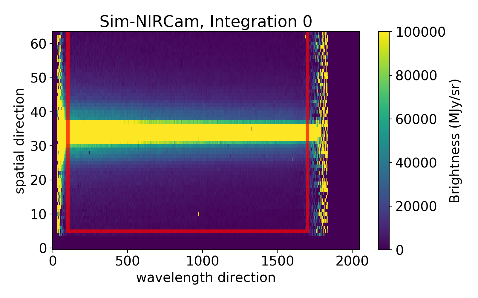
Everything outside of the box will be discarded and not used in the analysis.
For most datasets, any element of xwindow or ywindow can be set to None to use the full frame in that direction. However, for MIRI photometry, any element of xwindow or ywindow that is set to None will be replaced by a default based on the value of subarray_halfwidth (described below).
subarray_halfwidth
Only used if any element of xwindow or ywindow is set to None, and only used for MIRI photometry data. This sets the half-width of the xwindow, ywindow subarray in pixels and is centered on the approximate centroid position. For MIRI photometry, the default is 75 pixels, which is a good value for most datasets since the MIRI full frame images are very large and it is generally helpful and faster to zoom-in on the science target.
orders
Only used for NIRISS. List of spectral orders to be reduced.
trace_yoffset
Only used for NIRISS. PASTASOSS v1.2 doesn’t correctly compute the trace position for SUBSTRIP96 mode; therefore, we have to apply a manual offset in the cross-dispersion direction. The default is -12 pixels for SUBSTRIP96 and should be good to within a pixel or two. If you see in Fig. 3304 that the spectrum is not quite centered, you should adjust the trace_yoffset accordingly.
src_ypos
The user should only specify this parameter for NIRISS data. Spectral trace will be shifted to given vertical position. Must be same size as meta.orders.
src_pos_type
Determine the source position on the detector. Options: header, gaussian, weighted, max, or hst. The value ‘header’ uses the value of SRCYPOS in the FITS header.
record_ypos
Option to record the cross-dispersion trace position and width (if Gaussian fit) for each integration.
dqmask
Masks odd data quality (DQ) entries which indicate “Do not use” pixels following the jwst package documentation: https://jwst-pipeline.readthedocs.io/en/latest/jwst/references_general/references_general.html#data-quality-flags
expand
Super-sampling factor along cross-dispersion direction.
centroidtrim
Only used for HST analyses. The box width to cut around the centroid guess to perform centroiding on the direct images. This should be an integer.
centroidguess
Only used for HST analyses. A guess for the location of the star in the direct images in the format [x, y].
flatoffset
Only used for HST analyses. The positional offset to use for flatfielding. This should be formatted as a 2 element list with x and y offsets.
flatsigma
Only used for HST analyses. Used to sigma clip bad values from the flatfield image.
diffthresh
Only used for HST analyses. Sigma theshold for bad pixel identification in the differential non-destructive reads (NDRs).
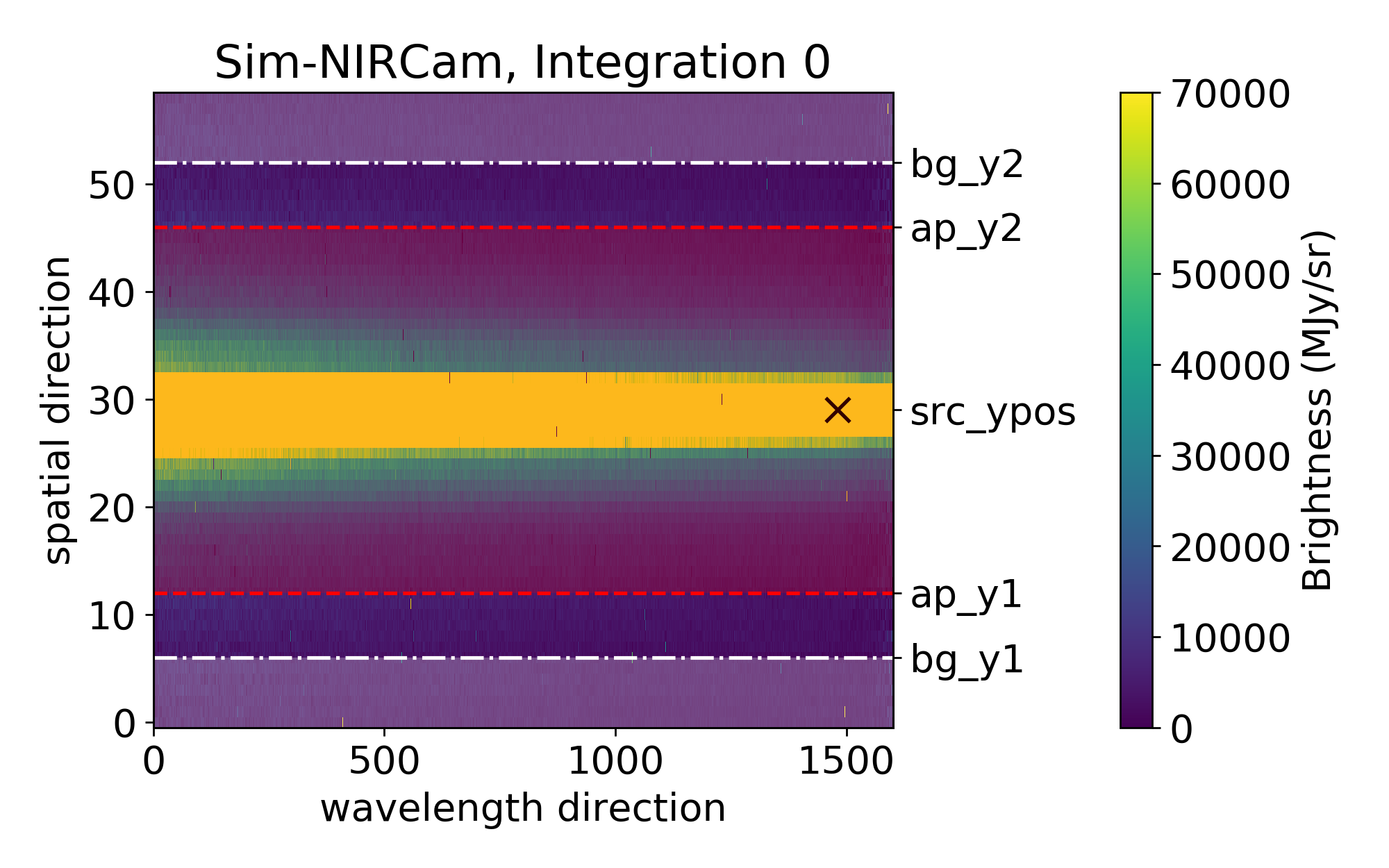
bg_hw & spec_hw
bg_hw and spec_hw set the background and spectrum aperture relative to the source position.
Let’s looks at an example with the following settings:
bg_hw    = 23
spec_hw  = 18
Looking at the fits file science header, we can determine the source position:
src_xpos = hdulist['SCI',1].header['SRCXPOS']-xwindow[0]
src_ypos = hdulist['SCI',1].header['SRCYPOS']-ywindow[0]
Let’s assume in our example that src_ypos = 29.
(xwindow[0] and ywindow[0] corrects for the trimming of the data frame, as the edges were removed with the xwindow and ywindow parameters)
The plot below shows you which parts will be used for the background calculation (shaded in white; between the lower edge and src_ypos - bg_hw, and src_ypos + bg_hw and the upper edge) and which for the spectrum flux calculation (shaded in red; between src_ypos - spec_hw and src_ypos + spec_hw).
If you want to try multiple values sequentially, you can provide a list in the format [Start, Stop, Step]; this will give you sizes ranging from Start to Stop (inclusively) in steps of size Step. For example, [10,14,2] tries [10,12,14], but [10,15,2] still tries [10,12,14]. If spec_hw and bg_hw are both lists, all combinations of the two will be attempted.
ff_outlier
Set False to use only the background region when searching for outliers along the time axis (recommended for deep transits). Set True to apply the outlier rejection routine to the full frame (works well for shallow transits/eclipses). Be sure to check the percentage of pixels that were flagged while ff_outlier = True; the value should be << 1% when bg_thresh = [5,5].
bg_thresh
Double-iteration X-sigma threshold for outlier rejection along time axis.
The flux of every full-frame or background pixel will be considered over time for the current data segment.
e.g: bg_thresh = [5,5]: Two iterations of 5-sigma clipping will be performed in time for every full-frame or background pixel. Outliers will be masked and not considered in the flux calculation.
bg_deg
Sets the degree of the column-by-column background subtraction. If bg_deg is negative, use the median background of entire frame. Set to None for no background subtraction. Also, best to emphasize that we’re performing column-by-column BG subtraction
The function is defined in S3_data_reduction.optspex.fitbg
Possible values:
bg_deg = None: No backgound subtraction will be performed.bg_deg < 0: The median flux value in the background area will be calculated and subtracted from the entire 2D Frame for this paticular integration.bg_deg => 0: A polynomial of degree bg_deg will be fitted to every background column (background at a specific wavelength). If the background data has an outlier (or several) which is (are) greater than 5 * (Mean Absolute Deviation), this value will be not considered as part of the background. Step-by-step:
Take background pixels of first column
Fit a polynomial of degree
bg_degto the background pixels.Calculate the residuals (flux(bg_pixels) - polynomial_bg_deg(bg_pixels))
Calculate the MAD (Mean Absolute Deviation) of the greatest background outlier.
If MAD of the greatest background outlier is greater than 5, remove this background pixel from the background value calculation. Repeat from Step 2. and repeat as long as there is no 5*MAD outlier in the background column.
Calculate the flux of the polynomial of degree
bg_deg(calculated in Step 2) at the spectrum and subtract it.
bg_method
Sets the method for calculating the sigma for use in outlier rejection. Options: ‘std’, ‘median’, ‘mean’. Defaults to ‘std’.
bg_row_by_row
Set True to perform row-by-row background subtraction (only useful for NIRCam).
bg_x1
The pixel number for the end of the left background region for row-by-row background subtraction. The background region goes from the left of the subarray to this pixel.
bg_x2
The pixel number for the start of the right background region for row-by-row background subtraction. The background region goes from this pixel to the right of the subarray.
p3thresh
Only important if bg_deg => 0 (see above). # sigma threshold for outlier rejection during background subtraction which corresponds to step 3 of optimal spectral extraction, as defined by Horne (1986).
p5thresh
Used during Optimal Extraction. # sigma threshold for outlier rejection during step 5 of optimal spectral extraction, as defined by Horne (1986). Default is 10. For more information, see the source code of optspex.optimize.
p7thresh
Used during Optimal Extraction. # sigma threshold for outlier rejection during step 7 of optimal spectral extraction, as defined by Horne (1986). Default is 10. For more information, see the source code of optspex.optimize.
fittype
Used during Optimal Extraction. fittype defines how to construct the normalized spatial profile for optimal spectral extraction. Options are: ‘smooth’, ‘meddata’, ‘wavelet’, ‘wavelet2D’, ‘gauss’, or ‘poly’. Using the median frame (meddata) should work well with JWST. Otherwise, using a smoothing function (smooth) is the most robust and versatile option. Default is meddata. For more information, see the source code of optspex.optimize.
window_len
Used during Optimal Extraction. window_len is only used when fittype = ‘smooth’ or ‘meddata’ (when computing median frame). It sets the length scale over which the data are smoothed. You can set this to 1 for no smoothing when computing median frame for fittype=meddata.
For more information, see the source code of optspex.optimize.
median_thresh
Used during Optimal Extraction. Sigma threshold when flagging outliers in median frame, when fittype=meddata and window_len > 1. Default is 5.
prof_deg
Used during Optimal Extraction. prof_deg is only used when fittype = ‘poly’. It sets the polynomial degree when constructing the spatial profile. Default is 3. For more information, see the source code of optspex.optimize.
iref
Only used for HST analyses. The file indices to use as reference frames for 2D drift correction. This should be a 1-2 element list with the reference indices for each scan direction.
curvature
Current options: ‘None’, ‘correct’. Using ‘None’ will not use any curvature correction and is strongly recommended against for instruments with strong curvature like NIRSpec/G395. Using ‘correct’ will bring the center of mass of each column to the center of the detector and perform the extraction on this straightened trace. If using ‘correct’, you should also be using fittype = ‘meddata’.
interp_method
Only used for photometry analyses. Interpolate bad pixels. Options: None (if no interpolation should be performed), linear, nearest, cubic
oneoverf_corr
Only used for photometry analyses. The NIRCam detector exhibits 1/f noise along the long axis. Furthermore, each amplifier area (which are all 512 columns in length) has its own 1/f characteristics. Correcting for the 1/f effect will improve the quality of the final light curve. So, performing this correction is advised if it has not been done in any of the previous stages. The 1/f correction in Stage 3 treats every amplifier region separately. It does a row by row subtraction while avoiding pixels close to the star (see oneoverf_dist). “oneoverf_corr” sets which method should be used to determine the average flux value in each row of an amplifier region. Options: None, meanerr, median. If the user sets oneoverf_corr = None, no 1/f correction will be performed in S3. meanerr calculates a mean value which is weighted by the error array in a row. median calculated the median flux in a row.
oneoverf_dist
Only used for photometry analyses. Set how many pixels away from the centroid should be considered as background during the 1/f correction. E.g., Assume the frame has the shape 1000 in x and 200 in y. The centroid is at x,y = 400,100. Assume, oneoverf_dist has been set to 250. Then the area 0-150 and 650-1000 (in x) will be considered as background during the 1/f correction. The goal of oneoverf_dist is therefore basically to not subtract starlight during the 1/f correction.
centroid_method
Only used for photometry analyses. Selects the method used for determining the centroid position (options: fgc or mgmc). For it’s initial centroid guess, the ‘mgmc’ method creates a median frame from each batch of integrations and performs centroiding on the median frame (with the exact centroiding method set by the centroid_tech parameter). For each integration, the ‘mgmc’ method will then crop out an area around that guess using the value of ctr_cutout_size, and then perform a second round of centroiding to measure how the centroid moves over time. The ‘fgc’ method is the legacy centroiding method and is not currently recommended.
ctr_guess
Optional, and only used for photometry analyses. An initial guess for the [x, y] location of the star that will replace the default behavior of first doing a full-frame Gaussian centroiding to get an initial guess. If set to ‘fits’, the code will use the approximate centroid position information contained in the FITS header as an starting point. If set to None, the code will first perform centroiding on whole frame (which can sometimes fail).
ctr_cutout_size
Only used for photometry analyses. For the ‘fgc’ and ‘mgmc’ methods this parameter is the amount of pixels all around the guessed centroid location which should be used for the more precise second centroid determination after the coarse centroid calculation. E.g., if ctr_cutout_size = 10 and the centroid (as determined after coarse step) is at (200, 200) then the cutout will have its corners at (190,190), (210,210), (190,210) and (210,190). The cutout therefore has the dimensions 21 x 21 with the centroid pixel (determined in the coarse centroiding step) in the middle of the cutout image.
centroid_tech
Only used for photometry analyses. The centroiding technique used if centroid_method is set to mgmc. The options are: com, 1dg, 2dg. The recommended technique is com (standing for Center of Mass). More details about the options can be found in the photutils documentation at https://photutils.readthedocs.io/en/stable/centroids.html.
gauss_frame
Only used for photometry analyses. Half-width of the pixel box centered around the centroid measurement to include in estimating gaussian width of the PSF. Options: this should be set to something larger than your expected PSF size; ~100 should work for defocused NIRCam photometry, and ~15 for MIRI photometry.
phot_method
Only used for photometry analyses. The method used to do photometric extraction. Options: ‘photutils’ (aperture photometry using photutils), ‘poet’ (aperture photometry using code from POET), or ‘optimal’ (for optimal photometric extraction).
aperture_edge
Only used for photometry analyses. Specifies how to treat pixels near the edge of the aperture. Options are ‘center’ (each pixel is included only if its center lies within the aperture), or ‘exact’ (each pixel is weighted by the fraction of its area that lies within the aperture).
aperture_shape
Only used for photometry analyses. Specifies the shape of the extraction aperture. If phot_method is photutils or optimal: circle, ellipse, or rectangle. If phot_method is poet: circle or hexagon. Used to set both the object aperture shape and the sky annulus shape. Hexagonal apertures may better match the shape of the JWST primary mirror for defocused NIRCam photometry.
moving_centroid
Only used for photometry analyses. If False (recommended), the aperture will stay fixed on the median centroid location. If True, the aperture will track the moving centroid.
skip_apphot_bg
Only used for photometry analyses. Skips the background subtraction in the aperture photometry routine. If the user does the 1/f noise subtraction during S3, the code will subtract the background from each amplifier region. The aperture photometry code will again subtract a background flux from the target flux by calculating the flux in an annulus in the background. If the user wants to skip the annular background subtraction step, skip_apphot_bg has to be set to True.
photap
Only used for photometry analyses. Size of photometry aperture in pixels. If aperture_shape is ‘circle’, then photap is the radius of the circle. If aperture_shape is ‘hexagon’, then photap is the radius of the circle circumscribing the hexagon. If aperture_shape is ‘rectangle’, then photap is the half-width of the rectangle along the x-axis. If the center of a pixel is not included within the aperture, it is being considered. If you want to try multiple values sequentially, you can provide a list in the format [Start, Stop, Step]; this will give you sizes ranging from Start to Stop (inclusively) in steps of size Step. For example, [10,14,2] tries [10,12,14], but [10,15,2] still tries [10,12,14]. If skyin and/or skywidth are also lists, all combinations of the three will be attempted.
photap_b
Only used for photometry analyses. If aperture_shape is ‘ellipse’, then photap is the size of photometry aperture radius along the y-axis in units of pixels. If aperture_shape is ‘rectangle’, then photap is the half-width of the rectangle along the y-axis. This parameter can only be used if aperture_shape is ellipse or rectangle.
photap_theta
Only used for photometry analyses. The rotation angle of photometry aperture in degrees. This parameter can only be used if aperture_shape is ellipse or rectangle. The aperture is rotated about the center of the aperture.
skyin
Only used for photometry analyses. Inner sky annulus edge, in pixels. If aperture_shape is ‘circle’, then skyin is the radius of the circle. If aperture_shape is ‘hexagon’, then skyin is the radius of the circle circumscribing the hexagon. If you want to try multiple values sequentially, you can provide a list in the format [Start, Stop, Step]; this will give you sizes ranging from Start to Stop (inclusively) in steps of size Step. For example, [10,14,2] tries [10,12,14], but [10,15,2] still tries [10,12,14]. If photap and/or skywidth are also lists, all combinations of the three will be attempted.
skywidth
Only used for photometry analyses. The width of the sky annulus, in pixels. If you want to try multiple values sequentially, you can provide a list in the format [Start, Stop, Step]; this will give you sizes ranging from Start to Stop (inclusively) in steps of size Step. For example, [10,14,2] tries [10,12,14], but [10,15,2] still tries [10,12,14]. If photap and/or skyin are also lists, all combinations of the three will be attempted.
isplots_S3
Sets how many plots should be saved when running Stage 3. A full description of these outputs is available here: Stage 3 Output
nplots
Sets how many integrations will be used for per-integration figures (Figs 3301, 3302, 3303, 3307, 3501, 3505). Useful for in-depth diagnoses of a few integrations without making thousands of figures. If set to None, a plot will be made for every integration.
vmin
Optional. Sets the vmin of the color bar for Figure 3101. Defaults to 0.97.
vmax
Optional. Sets the vmax of the color bar for Figure 3101. Defaults to 1.03.
time_axis
Optional. Determines whether the time axis in Figure 3101 is along the y-axis (‘y’) or the x-axis (‘x’). Defaults to ‘y’.
testing_S3
If set to True only the last segment (which is usually the smallest) in the inputdir will be run. Also, only five integrations from the last segment will be reduced.
save_output
If set to True output will be saved as files for use in S4. Setting this to False is useful for quick testing
save_fluxdata
If set to True (the default if save_fluxdata is not in your ECF), then save FluxData outputs for debugging or use with other tools. Note that these can be quite large files and may fill your drive if you are trying many spec_hw,bg_hw pairs.
hide_plots
If True, plots will automatically be closed rather than popping up on the screen.
verbose
If True, more details will be printed about steps.
topdir + inputdir
The path to the directory containing the Stage 2 JWST data, or, for HST observations, the _ima FITS files (including both direct images and spectra) downloaded from MAST. Directories containing spaces should be enclosed in quotation marks.
topdir + outputdir
The path to the directory in which to output the Stage 3 JWST data and plots. Directories containing spaces should be enclosed in quotation marks.
topdir + time_file
Optional. The path to a file that contains the time array you want to use instead of the one contained in the FITS file. Directories containing spaces should be enclosed in quotation marks.
Stage 4
# Eureka! Control File for Stage 4: Generate Lightcurves

# Stage 4 Documentation: https://eurekadocs.readthedocs.io/en/latest/ecf.html#stage-4

# Number of spectroscopic channels spread evenly over given wavelength range
nspecchan       2           # Number of spectroscopic channels spread evenly over given wavelength range. Set to None to leave the spectrum unbinned.
compute_white   True        # Also compute the white-light lightcurve
s4_order        None        # For NIRISS, specify spectral order
wave_min        1.5         # Minimum wavelength. Set to None to use the shortest extracted wavelength from Stage 3.
wave_max        4.5         # Maximum wavelength. Set to None to use the longest extracted wavelength from Stage 3.
wave_input      None        # Full path to a txt file with pre-defined wavelength bins in two columns separated by whitespace.
allapers        False       # Run S4 on all of the apertures considered in S3? Otherwise will use newest output in the inputdir. With allapers=True, inputdir can use a glob pattern such as Stage3/S3_*_run*/ap5_bg* to run one aperture over all matching backgrounds.

# Manually mask pixel columns by index number
# mask_columns  []
mad_sigma       7       # The number of sigmas an unbinned MAD value must be from the rolling median (using mad_box_width) to be considered an outlier.  Outlier columns are masked.
mad_box_width   21      # The rolling median box width to use when computing whether a wavelength element's MAD is an outlier

# Parameters for drift correction of 1D spectra
recordDrift     False   # Set True to record drift/jitter in 1D spectra (always recorded if correctDrift is True)
correctDrift    False   # Set True to correct drift/jitter in 1D spectra (not recommended)

# Parameters for sigma clipping
clip_unbinned   False   # Whether or not sigma clipping should be performed on the unbinned 1D time series
clip_binned     True    # Whether or not sigma clipping should be performed on the binned 1D time series
sigma           10      # The number of sigmas a point must be from the rolling median to be considered an outlier
box_width       10      # The width of the box-car filter (used to calculated the rolling median) in units of number of data points
maxiters        5       # The number of iterations of sigma clipping that should be performed.
boundary        fill    # Use 'fill' to extend the boundary values by the median of all data points (recommended), 'wrap' to use a periodic boundary, or 'extend' to use the first/last data points
fill_value      mask    # Either the string 'mask' to mask the outlier values (recommended), 'boxcar' to replace data with the mean from the box-car filter, or a constant float-type fill value.

# Limb-darkening parameters
compute_ld      False   # Options: exotic-ld, spam, False
# Options for ExoTiC-LD
metallicity     0.1     # Metallicity of the star
teff            6000    # Effective temperature of the star in K
logg            4.0     # Surface gravity in log g
exotic_ld_direc /home/User/exotic-ld_data/ # Directory for ancillary files for exotic-ld, download from: https://zenodo.org/doi/10.5281/zenodo.6047317
exotic_ld_grid  stagger # You can choose from kurucz (or 1D), stagger (or 3D), mps1, or mps2 model grids, or custom (to use custom_si_grid below)
# custom_si_grid  /home/User/path/to/custom/stellar/intensity/profile  #Custom Stellar Intensity profile. For examples see Eureka/demos/JWST/Custom_Stellar_Intensity_Files
# exotic_ld_file  /home/User/exotic-ld_data/Custom_throughput_file.csv # Custom throughput file, for examples see Eureka/demos/JWST/Custom_throughput_files
# Options for SPAM
spam_file       /home/User/spam-ldcoeff-u1-u2.txt # Pre-generated file of SPAM limb-darkening values at high resolution

# Diagnostics
isplots_S4      3       # Generate few (1), some (3), or many (5) figures (Options: 1 - 5)
vmin            0.97    # Sets the vmin of the color bar for Figure 4101.
vmax            1.03    # Sets the vmax of the color bar for Figure 4101.
time_axis       'y'     # Determines whether the time axis in Figure 4101 is along the y-axis ('y') or the x-axis ('x')
hide_plots      True    # If True, plots will automatically be closed rather than popping up
verbose         True    # If True, more details will be printed about steps

# Project directory
topdir          /home/User/Data/JWST-Sim/NIRSpec/

# Directories relative to topdir
inputdir        Stage3    # The folder containing the outputs from Eureka!'s S3 or JWST's S3 pipeline (will be overwritten if calling S3 and S4 sequentially). With allapers=True, glob patterns can restrict the previous-stage folders, e.g. Stage3/S3_*_run*/ap5_bg*.
outputdir       Stage4
nspecchan
Number of spectroscopic channels spread evenly over given wavelength range. Set to None to leave the spectrum unbinned.
compute_white
If True, also compute the white-light lightcurve.
wave_min & wave_max
Start and End of the wavelength range being considered. Set to None to use the shortest/longest extracted wavelength from Stage 3.
wave_input
Path to a user supplied txt file with pre-defined wavelength bins. Two columns (separated by whitespace): first column is the lower edge of the wavelength bins and the second column is the upper edge of the wavelength bins.
allapers
If True, run S4 on all of the apertures considered in S3. Otherwise the code will use the only or newest S3 outputs found in the inputdir. To specify a particular S3 save file, ensure that “inputdir” points to the procedurally generated folder containing that save file (e.g. set inputdir to /Data/JWST-Sim/NIRCam/Stage3/S3_2021-11-08_nircam_wfss_ap10_bg10_run1/).
When allapers is True, inputdir can include glob-style patterns to restrict which previous-stage aperture/background folders are processed. For example, setting inputdir to Stage3/S3_*_run*/ap5_bg* and allapers to True runs Stage 4 for aperture 5 over all matching background settings.
mask_columns
List of pixel columns that should not be used when constructing a light curve. Absolute (not relative) pixel columns should be used. Figure 3102 is very helpful for identifying bad pixel columns.
recordDrift
If True, compute drift/jitter in 1D spectra (always recorded if correctDrift is True)
correctDrift
If True, correct for drift/jitter in 1D spectra.
drift_preclip
Ignore first drift_preclip points of spectrum when correcting for drift/jitter in 1D spectra.
drift_postclip
Ignore the last drift_postclip points of spectrum when correcting for drift/jitter in 1D spectra. None = no clipping.
drift_range
Trim spectra by +/- drift_range pixels to compute valid region of cross correlation when correcting for drift/jitter in 1D spectra.
drift_hw
Half-width in pixels used when fitting Gaussian when correcting for drift/jitter in 1D spectra. Must be smaller than drift_range.
drift_iref
Index of reference spectrum used for cross correlation when correcting for drift/jitter in 1D spectra. -1 = last spectrum.
sub_mean
If True, subtract spectrum mean during cross correlation (can help with cross-correlation step).
sub_continuum
Set True to subtract the continuum from the spectra using a highpass filter
highpassWidth
The integer width of the highpass filter when subtracting the continuum
clip_unbinned
Whether or not sigma clipping should be performed on the unbinned 1D time series
clip_binned
Whether or not sigma clipping should be performed on the binned 1D time series
sigma
Only used if sigma_clip=True. The number of sigmas a point must be from the rolling median to be considered an outlier
box_width
Only used if sigma_clip=True. The width of the box-car filter (used to calculated the rolling median) in units of number of data points
maxiters
Only used if sigma_clip=True. The number of iterations of sigma clipping that should be performed.
boundary
Only used if sigma_clip=True. Use ‘fill’ to extend the boundary values by the median of all data points (recommended), ‘wrap’ to use a periodic boundary, or ‘extend’ to use the first/last data points
fill_value
Only used if sigma_clip=True. Either the string ‘mask’ to mask the outlier values (recommended), ‘boxcar’ to replace data with the mean from the box-car filter, or a constant float-type fill value.
mad_sigma
The number of sigmas an unbinned MAD value must be from the rolling median (using mad_box_width) to be considered an outlier. Outlier columns are masked.
mad_box_width
The width of the box-car filter (used to calculated the rolling median) in units of number of wavelength elements. Used in calculating whether wavelength elements are outliers in the unbinned spectrum.
sum_reads
Only used for HST analyses. Should differential non-destructive reads be summed together to reduce noise and data volume or not.
compute_ld
Whether or not to compute limb-darkening coefficients using exotic-ld.
metallicity
Used by exotic-ld if compute_ld=True. The metallicity of the star.
teff
Used by exotic-ld if compute_ld=True. The effective temperature of the star in K.
logg
Used by exotic-ld if compute_ld=True. The surface gravity in log g.
exotic_ld_direc
Used by exotic-ld if compute_ld=True. The fully qualified path to the directory for ancillary files for exotic-ld, available for download at https://zenodo.org/doi/10.5281/zenodo.6047317.
exotic_ld_grid
Used by exotic-ld if compute_ld=True. You can choose from “kurucz” (or “1D”), “stagger” (or “3D”), “mps1”, or “mps2” model grids, if you’re using exotic-ld v3. For more details about these grids, see https://exotic-ld.readthedocs.io/en/latest/views/supported_stellar_grids.html.
You can also use “custom” for a custom stellar intensity grid specified through the custom_si_grid parameter.
exotic_ld_file
Used by exotic-ld as throughput input file. If none, exotic-ld uses throughput from ancillary files. Make sure that wavelength is given in Angstrom!
custom_si_grid
If exotic_ld_grid = custom, supply the fully qualified path to your stellar intensity grid file here.
isplots_S4
Sets how many plots should be saved when running Stage 4. A full description of these outputs is available here: Stage 4 Output
nplots
Sets how many integrations will be used for per-integration figures (Figs 4301 and 4302). Useful for in-depth diagnoses of a few integrations without making thousands of figures. If set to None, a plot will be made for every integration.
vmin
Optional. Sets the vmin of the color bar for Figure 4101. Defaults to 0.97.
vmax
Optional. Sets the vmax of the color bar for Figure 4101. Defaults to 1.03.
time_axis
Optional. Determines whether the time axis in Figure 4101 is along the y-axis (‘y’) or the x-axis (‘x’). Defaults to ‘y’.
hide_plots
If True, plots will automatically be closed rather than popping up on the screen.
verbose
If True, more details will be printed about steps.
topdir + inputdir
The path to the directory containing the Stage 3 JWST data. Directories containing spaces should be enclosed in quotation marks.
topdir + outputdir
The path to the directory in which to output the Stage 4 JWST data and plots. Directories containing spaces should be enclosed in quotation marks.
Stage 4cal
# Eureka! Control File for Stage 4cal: Calibrated Stellar Spectra

# Stage 4cal Documentation: https://eurekadocs.readthedocs.io/en/latest/ecf.html#stage-4cal

# Transit/Eclipse time
t0              110.810782      # BJD
time_offset     60000           # Optional; time offset

# Orbital parameters
rprs            0.07194         # Planet-star radius ratio
period          4.2344923       # Orbital period (in Days)
inc             87.799          # orbital inclination (in degrees)
ars             12.518          # Semi-major axis to stellar radius ratio
# Transit durations. When given, the orbital parameters are ignored.
# t14             None            # Total transit duration, from t1 to t4
# t23             None            # Full transit duration, from t2 to t3

# Light curve to be used before t1 and after t4 for the baseline flux,
# which includes flux from (t1 - base_dur) to t1 and t4 to (t4 + base_dur).
base_dur        0.1             # Days

# Outlier detection
smoothing       1000            # A good starting point is the number of datapoints (i.e. wavelengths).  A value of 0 will apply interpolation.
sigma_thresh    [4,4,4]         # Three rounds of 4-sigma clipping ([4,4,4])

# Diagnostics
isplots_S4cal   3               # Generate few (1), some (3), or many (5) figures (Options: 1 - 5)
nbin_plot       200             # The number of time bins that should be used for figure 4202
hide_plots      False           # If True, plots will automatically be closed rather than popping up

# Project directory
topdir          /home/User/Data/JWST-Sim/NIRSpec/

# Directories relative to topdir
inputdir        Stage3          # The folder containing the calibrated stellar spectra from Eureka!'s S3 pipeline
outputdir       Stage4cal
t0
Transit or eclipse midpoint (in days).
time_offset
Absolute time offset of time-series data (in days). Defaults to 0.
rprs
Planet-to-star radius ratio.
period
Orbital period (in days).
inc
Orbital inclination (in degrees).
ars
Ratio of the semimajor axis to the stellar radius, a/R*.
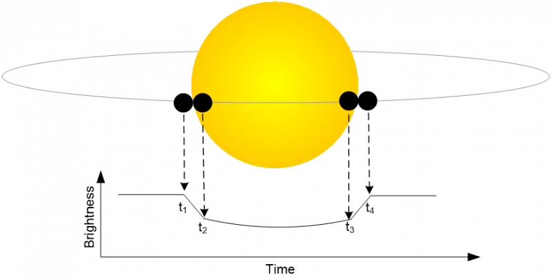
t14
Optional. Total transit duration, from t1 to t4 (see image below). The data points before t1 and after t4 are used to determine the out-of-transit baseline flux. When not given, t14 is computed using the orbital parameters above. When given, the orbital parameters are ignored.
t23
Optional. Full transit duration, from t2 to t3 (see image below). The data points between t2 and t3 are used to determine the in-transit flux. When not given, t23 is computed using the orbital parameters above. When given, the orbital parameters are ignored.
base_dur
Baseline duration used before t1 and after t4 (in days). Flux for the baseline region combines data points from (t1 - base_dur) to t1 and from t4 to (t4 + base_dur).
apcorr
Float specifying the multiplicative scalar necessary for correcting extracted imaging and spectroscopic photometry to the equivalent of an infinite aperture. By default is set to 1.0, but if set to this you will need to manually estimate the aperture correction value yourself by repeating the same procedure on one or (ideally) many calibrator targets and comparing the extracted flux to a stellar model. Aperture corrections are also hosted on CRDS, and you can learn more about the APCORR reference file here.
sigma_thresh
Sigma threshold when flagging outliers along the wavelength axis. Process is performed X times, where X is the length of the list. Defaults to [4, 4, 4].
isplots_S4cal
Sets how many plots should be saved when running Stage 4cal. Defaults to 3.
nbin_plot
The number of bins that should be used for figures 5104 and 5304. Defaults to 100.
s4cal_plotErrorType
The type of error bar to be plotted in Figure 4201. The currently supported options are: ‘stderr’ (the standard error of the mean), and ‘stddev’ (the standard deviation of the data). Defaults to ‘stderr’. The standard error of the mean is the standard deviation of the sample divided by the square root of the number of samples.
hide_plots
If True, plots will automatically be closed rather than popping up on the screen.
topdir + inputdir
The path to the directory containing the Stage 3 JWST data. Directories containing spaces should be enclosed in quotation marks.
topdir + outputdir
The path to the directory in which to output the Stage 4cal JWST data and plots. Directories containing spaces should be enclosed in quotation marks.
Stage 5
# Eureka! Control File for Stage 5: Lightcurve Fitting

# Stage 5 Documentation: https://eurekadocs.readthedocs.io/en/latest/ecf.html#stage-5

ncpu            4 # The number of CPU threads to use when running emcee or dynesty in parallel

multwhite       False  # Are you simultaneously fitting multiple white lightcurves?

allapers        False  # Run S5 on all of the apertures considered in S4? Otherwise will use newest output in the inputdir. With allapers=True, inputdir can use a glob pattern such as Stage4/S4_*_run*/ap5_bg* to run one aperture over all matching backgrounds.

# Manual clipping in time
manual_clip     None    # A list of lists specifying the start and end integration numbers for manual removal.

fit_par         ./S5_fit_par_template.epf   # What fitting epf do you want to use?
fit_method      [dynesty]                   #options are: lsq, emcee, dynesty, exoplanet, nuts (can list multiple types separated by commas)
run_myfuncs     [batman_tr,polynomial]      # options are: batman_tr, batman_ecl, catwoman_tr, sinusoid_pc, quasilambert_pc, poet_tr, poet_ecl, poet_pc, fleck_tr, starry, expramp, polynomial, step, xpos, ypos, xwidth, ywidth, lorentzian, damped_osc, and GP (can list multiple types separated by commas)
compute_ltt     False                       # options are: True (correct model for the light travel time effect), or False (ignore the light travel time effect)
force_positivity False                      # Optional boolean for sinusoid_pc and poet_pc models.  Set True to force positive phase variations.
# pixelsampling   False                       # Optional boolean for starry's phase curve and/or eclipse mapping model. Set to True to use starry's pixel-sampling method to ensure non-negative fluxes across the planet. Set to False (default) or leave undefined if you want to use starry's spherical harmonic method and are okay with permitting negative fluxes or if you intend to use Eureka!'s sinusoid_pc, quasilambert_pc, or poet_pc methods
# ydeg            2                           # Integer specifying the spherical harmonic order to use with starry's phase curve and/or eclipse mapping model. This setting is mandatory if you set pixelsampling to True, otherwise the setting is optional and will be inferred from your EPF settings.
# oversample      3                           # Optional integer specifying the oversampling factor to be used when converting spherical harmonics to pixels when pixelsampling has been set to True.

# Limb darkening controls
# IMPORTANT: limb-darkening coefficients are not automatically fixed. Change them to 'fixed' in your .epf file if they should be fixed!
use_generate_ld      None  # use the generated limb-darkening coefficients from Stage 4? Options: exotic-ld, spam, None. For exotic-ld and spam, the limb-darkening laws available are linear, quadratic, 3-parameter and 4-parameter non-linear.
ld_file              None  # Fully qualified path to the location of a limb darkening file that you want to use
ld_file_white        None  # Fully qualified path to the location of a limb darkening file that you want to use for the white-light light curve (required if ld_file is not None and any EPF parameters are set to white_free or white_fixed).
recenter_ld_prior    True  # Set to True if you want your Gaussian prior on the 'free' limb-darkening coefficients to be centered around the model coefficients for each wavelength.

# Spot contrast models
# IMPORTANT: spot-contrast coefficients are not automatically fixed. Change them to 'fixed' in your .epf file if they should be fixed!
spotcon_file              None  # Fully qualified path to the location of a spot contrast model file that you want to use
spotcon_file_white        None  # Fully qualified path to the location of a spot contrast model file that you want to use for the white-light light curve (required if spotcon_file is not None and any EPF parameters are set to white_free or white_fixed).
recenter_spotcon_prior    True  # Set to True if you want your Gaussian prior on the 'free' spot-contrast coefficients to be centered around the model coefficients for each wavelength.

# General fitter
old_fitparams   None # filename relative to topdir that points to a fitparams csv to resume where you left off (set to None to start from scratch)

# lsq fitter
lsq_method      Powell  # The scipy.optimize.minimize optimization method to use
lsq_tol         1e-7    # The tolerance for the scipy.optimize.minimize optimization method
lsq_maxiter     None    # Maximum number of iterations to perform. Depending on the method each iteration may use several function evaluations. Set to None to use the default value

# emcee fitter
old_chain       None    # Output folder relative to topdir that contains an old emcee chain to resume where you left off (set to None to start from scratch)
lsq_first       True    # Initialize with an initial lsq call (can help shorten burn-in, but turn off if lsq fails). Only used if old_chain is None
run_nsteps      1000
run_nwalkers    200
run_nburn       500     # How many of run_nsteps should be discarded as burn-in steps

# dynesty fitter
run_nlive       'min'    # Must be > ndim * (ndim + 1) // 2
run_bound       'multi'
run_sample      'auto'
run_tol         0.01

# dynamic dynesty fitter (in addition to the dynesty fitter parameters)
run_dynamic     False   # If False, use only dynesty static fitter; if True, use dynamic dynesty fitter
run_nlive_batch 'auto'  # Number of live points per batch for dynamic nested sampling; use int or 'auto' for minimum safe default (max(25, run_nlive // 2)).
run_pfrac        0.5    # Fraction of samples from posterior vs prior during refinement; 0.5 is balanced, higher favors posterior precision, lower improves evidence precision.

# PyMC3 NUTS fitter
exoplanet_first False   # Initialize with an initial exoplanet optimizer call (generally not recommended, but can sometimes be helpful if your initial manual guess is quite poor)
tune            3000
draws           1500
chains          3
target_accept   0.85

#GP inputs
kernel_inputs   ['time'] #options: time
kernel_class    ['Matern32'] #options: ExpSquared, Matern32, Exp, RationalQuadratic for george, Matern32 for celerite (sums of kernels possible for george separated by commas)
GP_package      'celerite' #options: george, celerite

# Plotting controls
interp          False   # Should astrophysical model be interpolated (useful for uneven sampling like that from HST)

# Diagnostics
isplots_S5      5       # Generate few (1), some (3), or many (5) figures (Options: 1 - 5)
nbin_plot       None    # The number of bins that should be used for figures 5104 and 5304
hide_plots      True    # If True, plots will automatically be closed rather than popping up
verbose         True    # If True, more details will be printed about steps

# Project directory
topdir          /home/User/Data/JWST-Sim/NIRSpec/

# Directories relative to topdir
inputdir        Stage4   # The folder containing the outputs from Eureka!'s S4 pipeline (will be overwritten if calling S4 and S5 sequentially). With allapers=True, glob patterns can restrict the previous-stage folders, e.g. Stage4/S4_*_run*/ap5_bg*.
outputdir       Stage5

# inputdirlist    []       # A list of additional Stage 4 input folders to use in a joint white lightcurve fit (e.g., NIRSpec NRS1+NRS2, or NIRCam+MIRI). Only relevant if multwhite is set to True
ncpu
Integer. Sets the number of CPUs to use for multiprocessing Stage 5 fitting.
allapers
Boolean to determine whether Stage 5 is run on all the apertures considered in Stage 4. If False, will just use the most recent output in the input directory.
When allapers is True, inputdir can include glob-style patterns to restrict which previous-stage aperture/background folders are processed. For example, setting inputdir to Stage4/S4_*_run*/ap5_bg* and allapers to True runs Stage 5 for aperture 5 over all matching background settings.
multwhite
Boolean to determine whether to run a joint fit of multiple white light curves. If True, must use inputdirlist.
fit_par
Path to Stage 5 priors and fit parameter file.
verbose
If True, more details will be printed about steps.
fit_method
Fitting routines to run for Stage 5 lightcurve fitting. For standard numpy functions, this can be one or more of the following: [lsq, emcee, dynesty]. For theano-based differentiable functions, this can be one or more of the following: [exoplanet, nuts] where exoplanet uses a gradient based optimization method and nuts uses the No U-Turn Sampling method implemented in PyMC3.
run_myfuncs
Determines the astrophysical and systematics models used in the Stage 5 fitting. For standard numpy functions, this can be one or more (separated by commas) of the following: [batman_tr, batman_ecl, harmonica_tr, catwoman_tr, fleck_tr, poet_tr, poet_ecl, sinusoid_pc, quasilambert_pc, expramp, hstramp, polynomial, step, xpos, ypos, xwidth, ywidth, lorentzian, damped_osc, common_mode, GP]. For theano-based differentiable functions, this can be one or more of the following: [starry, sinusoid_pc, quasilambert_pc, expramp, hstramp, polynomial, step, xpos, ypos, xwidth, ywidth], where starry replaces both the batman_tr and batman_ecl models and offers a more complicated phase variation model than sinusoid_pc that accounts for eclipse mapping signals. The POET transit and eclipse models assume a symmetric transit shape and, thus, are best-suited for planets with small eccentricities (e < 0.2). POET has a fast implementation of the 4-parameter limb darkening model that is valid for small planets (Rp/Rs < 0.1).
compute_ltt
Optional. Determines whether to correct the astrophysical model for the light travel time effect (True) or to ignore the effect (False). The light travel time effect is caused by the finite speed of light which means that the signal from a secondary eclipse (which occurs on the far side of the orbit) arrive later than would be expected if the speed of light were infinite. Unless specified, compute_ltt is set to True for batman_ecl and starry models but set to False for batman_tr models (since the light travel time is insignificant during transit).
num_planets
Optional. By default, the code will assume that you are only fitting for a single exoplanet. If, however, you are fitting signals from multiple planets simultaneously, you must set num_planets to the number of planets being fitted.
force_positivity
Optional boolean. Used by the sinusoid_pc and poet_pc models. If True, force positive phase variations (phase variations that never go below the bottom of the eclipse). Physically speaking, a negative phase curve is impossible, but strictly enforcing this can hide issues with the decorrelation or potentially bias your measured minimum flux level. Either way, use caution when choosing the value of this parameter.
common_mode_file
Optional. Fully qualified path to the location of the common-mode file that you want to use. This is usually the ECSV generated from a Stage 5 white LC fit.
common_mode_name
Required when common_mode_file is given. ECSV parameter name that represents the common-mode variations. This is usually GP or residuals.
pixelsampling
Optional boolean for starry’s phase curve and/or eclipse mapping model. Set to True to use starry’s pixel-sampling method to ensure non-negative fluxes across the planet and set priors on the pixel parameter(s) in your EPF. Set to False (default) or leave undefined if you want to use starry’s spherical harmonic method and are okay with permitting negative fluxes, or if you intend to use Eureka!’s sinusoid_pc, quasilambert_pc, or poet_pc methods.
ydeg
Optional integer. An integer specifying the spherical harmonic order to use with starry’s phase curve and/or eclipse mapping model. This setting is mandatory if you set pixelsampling to True, otherwise the setting is optional and will be inferred from your EPF settings.
oversample
Optional integer. Used by starry’s phase curve and/or eclipse mapping model when pixelsampling is set to True. The default value is 3 when pixelsampling is set to True which should generally suffice for most/all fits. For more details, read the documentation for the get_pixel_transforms function at https://starry.readthedocs.io/en/latest/SphericalHarmonicMap.
mutualOccultations
Optional boolean, only relevant for starry astrophysical models. If True (default), then the model will account for planet-planet occultations; if False, then the model will not include planet-planet occultations (and will likely take longer since each planet needs to be modelled separately).
manual_clip
Optional. A list of lists specifying the start and end integration numbers for manual removal. E.g., to remove the first 20 data points specify [[0,20]], and to also remove the last 20 data points specify [[0,20],[-20,None]]. If you want to clip the 10th integration, this would be index 9 since python uses zero-indexing. And the manual_clip start and end values are used to slice a numpy array, so they follow the same convention of inclusive start index and exclusive end index. In other words, to trim the 10th integrations, you would set manual_clip to [[9,10]].
Catwoman Convergence Parameters
The following two parameters can help in the case of convergence issues when using catwoman_tr.
catwoman_max_err
The max_err parameter used by catwoman; defaults to 1.0. For more information, see the relevant location of catwoman’s readthedocs page or the relevant location of catwoman’s API.
catwoman_fac
The fac parameter used by catwoman; defaults to None. For more information, see the relevant location of catwoman’s readthedocs page or the relevant location of catwoman’s API.
Limb Darkening Parameters
The following three parameters control the use of pre-generated limb darkening coefficients.
use_generate_ld
If you want to use the generated limb-darkening coefficients from Stage 4, use exotic-ld or spam. Otherwise, use None. Important: limb-darkening coefficients are not automatically fixed, change the limb darkening parameters to 'fixed' in the .epf file if they should be fixed instead of fitted! The limb-darkening laws available to exotic-ld and spam are linear, quadratic, 3-parameter, and 4-parameter (non-linear).
ld_file
If you want to use custom calculated limb-darkening coefficients, set to the fully qualified path to a file containing limb-darkening coefficients that you want to use. Otherwise, set to None. Note: this option only works if use_generate_ld=None. The file should be a plain .txt file with one column for each limb-darkening coefficient and one row for each wavelength range. Important: limb-darkening coefficients are not automatically fixed, change the limb darkening parameters to 'fixed' in the .epf file if they should be fixed instead of fitted!
ld_file_white
The same type of parameter as ld_file, but for the limb-darkening coefficients to be used for the white-light fit. This parameter is required if ld_file is not None and any of your EPF parameters are set to white_free or white_fixed. If no parameter is set to white_free or white_fixed, then this parameter is ignored.
recenter_ld_prior
If one of use_generate_ld or ld_file is not set to None, then this setting allows you apply a Normal prior centered on the limd-darkening model. To do this, you will need to keep the limb-darkening coefficients specified as 'free' in your EPF with your desired Gaussian standard deviation; any initial guess and Gaussian mean values you enter will be replaced with the values loaded in from the limb-darkeing model for each wavelength.
spotcon_file
If you want to use custom calculated spot-contrast coefficients, set to the fully qualified path to a file containing spot-contrast coefficients that you want to use. Otherwise, set to None. The file should be a plain .txt file with one column (or one column per spot if using starry) and one row for each wavelength bin. Important: spot-contrast coefficients are not automatically fixed, change the spot-contrast parameters to 'fixed' in the .epf file if they should be fixed instead of fitted!
spotcon_file_white
The same type of parameter as spotcon_file, but for the spot contrast coefficients to be used for the white-light fit. This parameter is required if spotcon_file is not None and any of your EPF parameters are set to white_free or white_fixed. If no parameter is set to white_free or white_fixed, then this parameter is ignored.
recenter_spotcon_prior
If spotcon_file is not set to None, then this setting allows you apply a Normal prior centered on the model provided by spotcon_file. To do this, you will need to keep the spot-contrast coefficients specified as 'free' in your EPF with your desired Gaussian standard deviation; any initial guess and Gaussian mean values you enter will be replaced with the values loaded in from spotcon_file for each wavelength.
GP parameters
The following parameters control part of the GP model (if listed in run_myfuncs).
kernel_inputs
Only used for fits with a GP. A list of the covariates to be used when fitting a GP to the model. At present, only GPs as a function of time are allowed, so this must be [‘time’]
kernel_class
Only used for fits with a GP. A list of the types of GP kernels to use. For the george GP package, this includes ExpSquared, Matern32, Exp, and RationalQuadratic. For the celerite package, this only includes Matern32. It is possible to sum multiple kernels possible for george by listing multiple kernels.
GP_package
Only used for fits with a GP. The Python GP package to use, with the options of ‘george’ or ‘celerite’.
useHODLR
Only used for fits with a GP. If True and GP_package is set to ‘george’, use the (potentially faster) HODLRSolver instead of the (more robust) BasicSolver.
Least-Squares Fitting Parameters
The following set the parameters for running the least-squares fitter.
lsq_method
Least-squares fitting method: one of any of the scipy.optimize.minimize least-squares methods. We recommend using Powell.
lsq_tolerance
Float to determine the tolerance of the scipy.optimize.minimize method.
lsq_maxiter
Integer. Maximum number of iterations to perform. Set to None to use the default value for the given scipy.optimize.minimize method.
Emcee Fitting Parameters
The following set the parameters for running emcee.
old_chain
Output folder containing previous emcee chains to resume previous runs. To start from scratch, set to None.
lsq_first
Boolean to determine whether to run least-squares fitting before MCMC. This can shorten burn-in but should be turned off if least-squares fails. Only used if old_chain is None.
run_nsteps
Integer. The number of steps for emcee to run.
run_nwalkers
Integer. The number of walkers to use.
run_nburn
Integer. The number of burn-in steps to run.
Dynesty Fitting Parameters
The following set the parameters for running dynesty. These options are described in more detail in: https://dynesty.readthedocs.io/en/latest/api.html#module-dynesty.dynesty
run_nlive
Integer or 'min'. Number of live points for dynesty to use. Should be at least greater than (ndim * (ndim + 1)) / 2, where ndim is the number of fitted parameters. For shared fits, multiply the number of free parameters by the number of wavelength bins specified in Stage 4.
For convenience, this can be set to 'min' to automatically use the minimum recommended value.
run_bound
The bounding method to use. Options are: ['none', 'single', 'multi', 'balls', 'cubes']
run_sample
The sampling method to use. Options are: ['auto', 'unif', 'rwalk', 'rstagger', 'slice', 'rslice', 'hslice']
run_tol
Float. The convergence tolerance for the dynesty run. The run will stop when the estimated contribution of the remaining prior volume to the total evidence falls below this threshold.
dynesty_checkpoint
Boolean. If True, dynesty will periodically write checkpoint files while running. These files are intended for resuming interrupted long runs and should generally be resumed with the same dynesty version.
dynesty_resume
Boolean. If True, dynesty will resume from an existing checkpoint file instead of starting a fresh sampler. Set old_dynesty_checkpoint to the previous checkpoint file or to the parent folder that contains Eureka’s standardized checkpoint file. The checkpoint should generally come from the same dynesty version.
dynesty_checkpoint_every
Float or integer. Number of seconds between dynesty checkpoint writes. Defaults to 600.
old_dynesty_checkpoint
String or None. Previous dynesty checkpoint file or parent folder, relative to topdir, used when dynesty_resume is True. If this points to a folder, Eureka will look inside that folder for the standardized fitter/channel-specific checkpoint filename.
dynesty_maxiter
Integer or None. Optional maximum number of dynesty iterations to run. Defaults to None.
dynesty_maxcall
Integer or None. Optional maximum number of likelihood calls for dynesty. Defaults to None.
For normal science runs, it is strongly recommended leaving both dynesty_maxiter and dynesty_maxcall
set to None so dynesty can run until its convergence criterion is satisfied. These parameters are
hard stop limits, and setting either one too low can stop the sampler before convergence, producing unreliable
posterior samples and evidence estimates. Finite values are mainly useful for debugging, smoke tests, benchmarking,
CI tests, or intentionally running only a partial fit.
Dynamic Nested Sampling Parameters
The following parameters control dynesty’s dynamic nested sampling behavior. These are only used if run_dynamic is set to True. Dynamic nested sampling adaptively allocates live points to focus more efficiently on the posterior distribution. More details are available in the dynesty documentation: https://dynesty.readthedocs.io/en/stable/dynamic.html
Dynamic nested sampling is typically preferred for complex or multimodal posteriors, as it adaptively allocates live points to focus more efficiently on the regions of interest.
It is generally more efficient for parameter estimation, especially when the posterior has sharp features or multiple peaks.
However, because it adds samples in batches based on runtime decisions, the estimated evidence (logZ) can vary more between runs.
Static nested sampling, on the other hand, uses a fixed number of live points from start to finish, which can make evidence estimates more stable and repeatable; this is particularly useful if you are comparing models using Bayes factors or need exact reproducibility.
If you are primarily focused on estimating parameters, dynamic sampling with a high run_pfrac (e.g., 0.8) is a good choice.
If you care most about comparing models based on their evidence, consider using static sampling or dynamic sampling with a lower run_pfrac (e.g., 0.1-0.3).
When run_dynamic = True, dynesty uses run_nlive to set the number of live points in the initial exploratory phase. The parameters run_nlive_batch and run_pfrac then control the behavior of refinement batches. Other static parameters such as run_bound, run_sample, and run_tol still apply and should be set as usual.
run_dynamic
Boolean. If True, dynesty will use its DynamicNestedSampler instead of NestedSampler. Dynamic nested sampling is often more efficient for complex or multimodal posteriors, as it adaptively refines high-posterior regions. If False, static nested sampling will be used with a fixed number of live points (run_nlive).
run_nlive_batch
Integer or 'auto'. The number of live points to allocate in each refinement batch during dynamic nested sampling. Controls how many new live points are used to zoom in on regions of high posterior probability.
Typical values range from one-half to equal the value of run_nlive. For example, if run_nlive = 200, a common value for run_nlive_batch would be 100-200.
If set to 'auto', a safe default of max(25, run_nlive // 2) is used.
run_pfrac
Float between 0 and 1 (exclusive). The fraction of samples to draw from the posterior distribution versus the prior during refinement. A higher value prioritizes detailed posterior exploration, while a lower value improves evidence (logZ) estimation.
Use run_pfrac = 0.5 for a balanced approach. Increase to 0.7-0.9 if you are primarily interested in posterior parameter estimation. If your goal is Bayesian model comparison, where precise estimation of the evidence (logZ) is important, consider lower values such as run_pfrac = 0.1-0.3.
NUTS Fitting Parameters
The following set the parameters for running PyMC3’s NUTS sampler. These options are described in more detail in: https://docs.pymc.io/en/v3/api/inference.html#pymc3.sampling.sample
exoplanet_first
Boolean to determine whether to run exoplanet optimizer before NUTS. This is generally not recommended, but it can sometimes be helpful if your initial manual guess is quite poor.
tune
Number of iterations to tune. Samplers adjust the step sizes, scalings or similar during tuning. Tuning samples will be drawn in addition to the number specified in the draws argument.
draws
The number of samples to draw. The number of tuned samples are discarded by default.
chains
The number of chains to sample. Running independent chains is important for some convergence statistics and can also reveal multiple modes in the posterior. If None, then set to either ncpu or 2, whichever is larger.
target_accept
Adapt the step size such that the average acceptance probability across the trajectories are close to target_accept. Higher values for target_accept lead to smaller step sizes. A default of 0.8 is recommended, but setting this to higher values like 0.9 or 0.99 can help with sampling from difficult posteriors. Valid values are between 0 and 1 (exclusive).
Plotting and Diagnostics
interp
Boolean to determine whether the astrophysical model is interpolated when plotted. This is useful when there is uneven sampling in the observed data.
isplots_S5
Sets how many plots should be saved when running Stage 5. A full description of these outputs is available here: Stage 5 Output
nbin_plot
The number of bins that should be used for figures 5104 and 5304. Defaults to 100.
hide_plots
If True, plots will automatically be closed rather than popping up on the screen.
topdir + inputdir
The path to the directory containing the Stage 4 JWST data. Directories containing spaces should be enclosed in quotation marks.
topdir + inputdirlist
List of paths to the additional white lightcurve directories. topdir + inputdir contains the first white lightcurve, while this list contains additional lightcurves. Each item must be enclosed in quotation marks. Ensure there are brakets around the list.
For example, to simultaneously fit white light curves of WASP-39b from NIRSpec/G395H NRS1 & NRS2 and MIRI/LRS, you might set topdir to /home/User/Data/WASP-39b, inputdir to NIRSpec/NRS1/Stage4_white/S4_2024-06-04_nirspec_fs_template_run1/, and inputdirlist to ['NIRSpec/NRS2/Stage4_white/S4_2024-06-04_nirspec_fs_template_run1/','MIRI/LRS/Stage4_white/S4_2024-06-04_miri_lrs_template_run1/'].
topdir + outputdir
The path to the directory in which to output the Stage 5 JWST data and plots. Directories containing spaces should be enclosed in quotation marks.
Stage 5 Fit Parameters
Warning
The Stage 5 fit parameter file has the file extension .epf, not .ecf. These have different formats, and are not interchangeable.
This file describes the transit/eclipse and systematics parameters and their prior distributions. Each line describes a new parameter, with the following basic format:
Name Value Free PriorPar1 PriorPar2 PriorType
Name defines the specific parameter being fit for. When fitting for multiple channels simultaneously, you can add optionally add _ch# after the parameter (e.g., rprs, rprs_ch1, rprs_ch2, etc.) to set channel-specific priors; if you don’t manually set a different prior for each channel, the code will default to the prior for the 0th channel (e.g., rprs).
Available fitting parameters are:
- Transit and Eclipse Depth Parameters
rporrprs- planet-to-star radius ratio, for all transit models.
a#and/orb#- nth harmonic amplitude (Harmonica only). Adda1to fit different morning/evening limbs. Addb1to fit different north/south limbs. Higher-order harmonics (up ton=3) are also available. We recommend starting withrpanda1as free parameters. See the Harmonica documentation for a detailed description of transmission strings and the Fourier series used to parameterize them.
fporfpfs- planet-to-star flux ratio, for the eclipse models.
rp2orrprs2- an additional planet-to-star radius ratio for use with the catwoman transit model to model transit limb-asymmetries.
phi- the angle (in degrees) of the line separating the semi-circles defined byrpandrp2in the catwoman transit model. Ifphiis set to 90 degrees (the parameter’s default value), therpis the trailing hemisphere andrp2is the leading hemisphere. Ifphiis set to 0, thenrpis the northern hemisphere andrp2is the southern hemisphere.When fitting for multiple planets, add
_pl#after the parameter (e.g.,rprs,rprs_pl1,rprs_pl2, etc.). This also applies to the planetaty orbital parameters below. Also be sure to set thenum_planetsparameter in your ECF (not EPF) to specify the number of planets being modelled simultaneously.
- Orbital Parameters
per- orbital period (in days)
t0- transit time (in the same units as your input data - most likely BMJD_TDB)
time_offset- (optional), the absolute time offset of your time-series data (in days)
inc- orbital inclination (in degrees)
OR,
b- orbital impact parameter (unitless)
aorars- a/R*, the ratio of the semimajor axis to the stellar radius
eccandw- orbital eccentricity (unitless) and argument of periapsis (degrees)
OR,
ecoswandesinw- the orbital eccentricity and argument of periapsis converted into a basis in which you can apply [0,1] uniform priors without biasing your results away fromecc ~ 0.
t_secondary- (optional) time of secondary eclipse
Rs- the host star’s radius in units of solar radii.This parameter is recommended for batman_ecl and poet_ecl fits as it allows for a conversion of a/R* to physical units in order to account for light travel time. If not provided for batman_ecl fits, the finite speed of light will not be accounted for. Fits with the starry model require that
Rsbe provided as starry always uses physical units. This parameter should be set tofixedunless you really want to marginalize overRs.
- Sinusoidal Phase Curve Parameters
The sinusoid_pc phase curve model for the standard numpy models allows for the inclusion of up to four sinusoids into a single phase curve. The theano-based differentiable functions allow for any number of sinusoids.
AmpCos1- Amplitude of the first cosine with one peak near eclipse (orbital phase 0.5). The units are in fractions of the eclipse depth.
AmpSin1- Amplitude of the first sine with one peak near quadrature at orbital phase 0.75. The units are in fractions of the eclipse depth.
AmpCos2- Amplitude of the second cosine with two peaks near eclipse (orbital phase 0.5) and transit (orbital phase 0). The units are in fractions of the eclipse depth.
AmpSin2- Amplitude of the second sine with two peaks near quadrature at orbital phases 0.25 and 0.75. The units are in fractions of the eclipse depth.
- POET Phase Curve Parameters
The poet_pc phase curve model allows for the inclusion of up to two sinusoids into a single phase curve, but allows for the inclusion of offsets, thus making it functionally identical to sinusoid_pc.
cos1_amp- Amplitude of the first cosine with period, per. The units are in fractions of the eclipse depth.
cos1_off- Offset (in degrees) of the first cosine, relative to the time of secondary eclipse.
cos2_amp- Amplitude of the second cosine with period, per/2. The units are in fractions of the eclipse depth.
cos2_off- Offset (in degrees) of the second cosine, relative to the time of secondary eclipse.
- Quasi-Lambertian Phase Curve Parameters
The quasilambert_pc phase curve model allows modelling of thermal phase variations of airless planets or reflected light due to aerosols. The phase function follows the formalism of Agol+2007 and has the form
np.abs(np.cos((phi+quasi_offset*np.pi/180)/2))**quasi_gamma, wherephiis the orbital phase in radians with a value of zero at mid-eclipse.
quasi_gamma- The exponential coefficient of the quasi-Lambertian phase function. A true Lambertian phase function is closely approximated with a value of 3.285. A value below 2 produces unphysical results.
quasi_offset- Offset in degrees East (i.e., before eclipse) of the quasi-Lambertian phase function, relative to the time of secondary eclipse.
- Starry Phase Curve and Eclipse Mapping Parameters
The starry model allows for the modelling of an arbitrarily complex phase curve by fitting the phase curve using spherical harmonics terms for the planet’s brightness map
You can use
Yl_m- Spherical harmonic coefficients normalized by the Y0_0 term wherelandmshould be replaced with integers.
lcan be any integer greater than or equal to 1, andmcan be any integer between-lto+l. For example, theY1_0term fits for the sub-stellar to anti-stellar brightness ratio (comparable toAmpCos1), theY1_1term fits for the East–West brightness ratio (comparable to-AmpSin1), and theY1_-1term fits for the North–South pole brightness ratio (undetectable using phase variations, but potentially detectable using eclipse mapping). TheY0_0term cannot be fit directly but is instead fit through the more observablefpterm which is composed of theY0_0term and the square of therpterm.OR, you can use
pixel#- Spherical harmonic coefficients converted into pixel space as described at https://starry.readthedocs.io/en/latest/notebooks/PixelSampling/; using pixel sampling can allow you to impose a physicality constraint that the planetary flux does not go negative anywhere.Replace the # with the pixel number (starting with just
pixelfor pixel #0). The number of pixels for any given fit is a function of the spherical harmonic order (set byydegin your ECF) as well as the oversampling factor (set byoversamplein your ECF). In most cases, you will just want to set the same prior for all pixels, regardless of the spherical harmonic order or oversampling factor; the simplest way to do this is to just set a prior for thepixelparameter in your EPF which will then automatically be copied to all other pixels not specified in your EPF. Since the numerical values of the pixels are normalized to give the eclipse depth specified byfp, it is recommended to impose a uniform prior spanning the range 0–1 for all pixels.
- Limb Darkening Parameters
limb_dark- The limb darkening model to be used.Options are:
['uniform', 'linear', 'quadratic', 'kipping2013', 'squareroot', 'logarithmic', 'exponential', '4-parameter'].uniformlimb-darkening has no parameters,linearhas a single parameteru1,quadratic,kipping2013,squareroot,logarithmic, andexponentialhave two parametersu1, u2, and4-parameterhas four parametersu1, u2, u3, u4.
- Stellar Variability Parameters, Flares
lor_amp,lor_amp_lhs,lor_amp_rhs- The amplitude of the Lorentzian. For a single basline/amplitude, uselor_amp. For different baselines/amplitudes, uselor_amp_lhsandlor_amp_rhsfor the left and right hand sides, respectively.
lor_hwhm,lor_hwhm_lhs,lor_hwhm_rhs- The half-width at half maximum. For a symmetric Lorentzian, uselor_hwhm. For an asymmetric Lorentzian, uselor_hwhm_lhsandlor_hwhm_rhsfor the left and right hand sides, respectively.
lor_t0- The midpoint of the Lorentzian.
lor_power- The exponent,p, in a modified Lorentzian with functional form,1/(1+x^p). The default is 2, representing a standard Lorentzian.The Lorentzian model is defined as:
lorentzian = 1 + lor_amp/(1 + x**lor_power), such thatx = 2*(time-lor_t0)/lor_hwhm.
- Stellar Variability Parameters, Quasi-Periodic Pulsations
osc_amp- The initial amplitude of the sinusoidal function.
osc_amp_decay- The rate of amplitude damping.
osc_per- The initial period of the sinusoidal function.
osc_per_decay- The rate of period damping.
osc_t0- The start time of the oscillations. The models returns unity flux for all times beforeosc_t0.
osc_t1- This offset determined the start phase of the sinusoidal function.The time-dependent amplitude and period are defined as follows:
amp = osc_amp * np.exp(-osc_amp_decay * (time - osc_t0))andper = osc_per * np.exp(-osc_per_decay * (time - osc_t0)). The damped oscillator model is then defined as:osc = 1 + amp * np.sin(2 * np.pi * (time - osc_t1) / per). Note thatosc[time < osc_t0] = 1.
- Star Spot Parameters (using fleck_tr or starry)
spotstari- The stellar inclination in degrees. Only matters when the star is rotating so that spots move appropriately relative to the planet, do not need to set unless you’re accounting for stellar rotation (fleck slow mode, seespotrotbelow), then place priors based on inclination measurements of the stellar inclination. Recommend using fast mode if this is not known! If running multwhite or shared fits, this should be set to ‘shared’.
spotrot- The stellar rotation rate in days. For fleck, only assign if you’d like to run in slow mode! (In slow mode the star rotates and spots move appropriately. Otherwise, Eureka! will use fleck’s fast mode which assumes the stellar rotation is >> transit time and spots are stationary). If running multwhite or shared fits, this should be set to ‘shared’.
spotcon#- The spot contrast ratio. Fleck only supports a single contrast ratio that is used for all spots, but for starry assign one value per spot. Replace the # with the spot number (starting with nothing (justspotcon) for spot #0, and thenspotcon1for the next spot)
spotrad#- The spot radius relative to the star. Replace the # with the spot number (starting with nothing (justspotrad) for spot #0, and thenspotrad1for the next spot)
spotlat#- The spot latitude in degrees. 0 is the center of the star (at time=0 if you have set thespotrotparameter). Replace the # with the spot number (starting with nothing (justspotlat) for spot #0, and thenspotlat1for the next spot)
spotlon#- The spot longitude in degrees. 0 is the center of the star (at time=0 if you have set thespotrotparameter). Replace the # with the spot number (starting with nothing (justspotlon) for spot #0, and thenspotlon1for the next spot)Fleck specific parameters: -
spotnpts- The number of temporal points to evalaute at. ~200-500 is good.Starry specific parameters: -
spotnpts- The degree of spherical harmonics on the star (ydeg). ~30 is needed to appropriately model the spot.
- Systematics Parameters. Depends on the model specified in the Stage 5 ECF.
c0--c9- Coefficients for 0th to 9th order polynomials.The polynomial coefficients are numbered as increasing powers (i.e.
c0a constant,c1linear, etc.). The x-values of the polynomial are the time with respect to the mean of the time of the lightcurve time array. Polynomial fits should include at leastc0for usable results.
r0--r1andr2--r3- Coefficients for the first and second exponential ramp models.The exponential ramp model is defined as follows:
r0*np.exp(-r1*time_local) + r2*np.exp(-r3*time_local) + 1, wherer0--r1describe the first ramp, andr2--r3the second.time_localis the time relative to the first frame of the dataset. If you only want to fit a single ramp, you can omitr2--r3or set them as fixed to0.
h0--h5- Coefficients for the HST exponential + polynomial ramp model.The HST ramp model is defined as follows:
1 + h0*np.exp(-h1*time_batch) + h2*time_batch + h3*time_batch**2, whereh0--h1describe the exponential ramp per HST orbit,h2--h3describe the polynomial (up to order two) per HST orbit,h4is the orbital period of HST (in the same time units as the data, usually days), andh5is the time offset when computingtime_batch. A good starting point forh4is 0.066422 days andh5is 0.03 days.time_batch = (time_local-h5) % h4. If you want to fit a linear trend in time, you can omith3or fix it to0.
step0andsteptime0- The step size and time for the first step function (useful for removing mirror segment tilt events).For additional steps, simply increment the integer at the end (e.g.
step1andsteptime1). The change in flux is relative to the flux from the previous step.
xpos- Coefficient for linear decorrelation against drift/jitter in the x direction (spectral direction for spectroscopy data).
xwidth- Coefficient for linear decorrelation against changes in the PSF width in the x direction (cross-correlation width in the spectral direction for spectroscopy data).
ypos- Coefficient for linear decorrelation against drift/jitter in the y direction (spatial direction for spectroscopy data).
ywidth- Coefficient for linear decorrelation against changes in the PSF width in the y direction (spatial direction for spectroscopy data).
cm1andcm2- Coefficients for the 1st and 2nd order common-mode systematics.The common-mode systematics model is defined as follows:
1 + cm1*cm_flux + cm2*cm_flux**2, wherecm1andcm2are common-mode amplitude parameters andcm_fluxrepresents the common-mode flux variations. Thecm_fluxarray is read in fromcommon_mode_file(generated from a Stage 5 white light curve fit) and uses mean-subtracted values from the ECSV parameter namecommon_mode_name(e.g.,GPorresiduals).
Aandm- The natural logarithm (ln) of the covariance amplitude and lengthscale to use for the GP model specified in your Stage 5 ECF.Significant care should be used when specifying the priors on these parameters as an excessively flexible GP model may end up competing with your astrophysical model. That said, there are no hard and fast rules about what your priors should be, and you will need to experiment to find what works best. If there are multiple kernels that are being added, the second kernel’s parameters will be
A1andm1, and so on.White Noise Parameters - options are
scatter_multfor a multiplier to the expected noise from Stage 3 (recommended), orscatter_ppmto directly fit the noise level in ppm.
Free determines whether the parameter is fixed, free, white_fixed, white_free, independent, or shared.
fixed parameters are fixed in the fitting routine and not fit for.
free parameters are fit for according to the specified prior distribution, independently for each wavelength channel.
white_fixed and white_free parameters are first fit using free on the white-light light curve to update the prior for the parameter, and then treated as fixed or free (respectively) for the spectral fits.
shared parameters are fit for according to the specified prior distribution, but are common to all wavelength channels.
independent variables set auxiliary functions needed for the fitting routines.
The PriorType can be U (Uniform), LU (Log Uniform), or N (Normal). If U/LU, then PriorPar1 and PriorPar2 are the lower and upper limits of the prior distribution. If N, then PriorPar1 is the mean and PriorPar2 is the stadard deviation of the Gaussian prior.
Here’s an example fit parameter file:
# Stage 5 Fit Parameters Documentation: https://eurekadocs.readthedocs.io/en/latest/ecf.html#stage-5-fit-parameters


# Name       Value         Free?          PriorPar1    PriorPar2    PriorType
# "Free?" can be free, fixed, white_free, white_fixed, shared, or independent
# PriorType can be U (Uniform), LU (Log Uniform), or N (Normal).
# If U/LU, PriorPar1 and PriorPar2 represent lower and upper limits of the parameter/log(the parameter).
# If N, PriorPar1 is the mean and PriorPar2 is the standard deviation of a Gaussian prior.
#-------------------------------------------------------------------------------------------------------
# ------------------
# ** Transit/eclipse parameters **
# ------------------
rp           0.148          'free'         0            0.5          U
# fp           0.008          'free'         0            0.5          U

# ------------------
# ** Orbital parameters **
# ------------------
per          4.055259       'free'         4.055259     1e-5         N
t0           57394.524      'free'         57394.524    0.05         N
inc          87.83          'free'         87.83        0.25         N
a            10.9           'free'         10.9         1            N
ecc          0.0            'fixed'        0            1            U
w            90.            'fixed'        0            180          U
# t_secondary  0.25           'free'         0.25         0.05         N
# Rs           0.12           'fixed'

# ----------------------
# ** Sinusoid_pc phase curve parameters **
# ----------------------
# AmpCos1      0.4           'free'         0            1            U
# AmpSin1      0.01          'free'         -1           1            U
# AmpCos2      0.01          'free'         -1           1            U
# AmpSin2      0.01          'free'         -1           1            U
# ----------------------
# ** POET_pc phase curve parameters **
# ----------------------
# cos1_amp     0.4           'free'         0            1            U
# cos1_off     0.00          'free'         -180         180          U
# cos2_amp     0.1           'free'         0            1            U
# cos2_off     0.00          'free'         0            180          U
# ----------------------
# ** quasilambert_pc phase curve parameters **
# ----------------------
# quasi_gamma  4             'free'         2            40           U
# quasi_offset 0             'free'         -90          90           U
# ----------------------
# ** starry spherical harmonic phase curve parameters **
# ----------------------
# Y1-1         0             'free'         -1           1            U
# Y10          0.5           'free'         -1           1            U
# Y11          0.1           'free'         -1           1            U
# ----------------------
# ** starry pixel-sampling phase curve parameters **
# ----------------------
# pixel        0.5           'free'         0            1            U

# -------------------------
# ** Limb darkening parameters **
# For BATMAN, choose limb_dark from ['uniform', 'linear', 'quadratic', 'kipping2013', 'squareroot', 'logarithmic', 'exponential','3-parameter', '4-parameter']
# For POET, choose limb_dark from ['uniform', 'linear', 'quadratic', '4-parameter']
# When using generated limb-darkening coefficients from exotic-ld or spam, choose from ['linear', 'quadratic', '3-parameter', '4-parameter'] and set their state to 'fixed' or use `recenter_ld_prior`.
# -------------------------
limb_dark   'kipping2013'   'independent'
u1          0.2             'free'          0           1           U
u2          0.2             'free'          0           1           U

# -------------------------
# ** Stellar variability parameters **
# A modified Lorentzian model can be used to fit stellar flares
# A damped oscillator model can be used to fit quasi-periodic pulsations
# -------------------------
# lor_amp_lhs     0.03    'free'          0            0.1            U
# lor_amp_rhs     0.03    'free'          0            0.1            U
# lor_hwhm_lhs    0       'fixed'         0            0.1            U
# lor_hwhm_rhs    1e-5    'free'          0            0.1            U
# lor_t0          0.3163  'free'          0.3160       0.3166         U
# lor_power       0.7     'free'          0.1          2              U

# osc_amp         0.0003  'free'          0            0.01           U
# osc_amp_decay   1       'free'          0            20             U
# osc_per         0.03    'free'          0            0.1            U
# osc_per_decay   0.      'fixed'         0            10             U
# osc_t0          0.3163  'fixed'         0            1              U
# osc_t1          0.3163  'free'          0.3          0.4            U

# ------------------
# ** Star Spot parameters **
# Each spot needs rad, lat, lon. See docs for details!
# For fleck: can only have one spot contrast (spotcon), spotnpts is the number of temporal points to evaluate at (~200-500)
# For starry: assign one spotcon per spot (spotcon, spotcon1, etc), spotnpts is the ydeg of the star map (~30)
# ------------------
# spotstari    90       'fixed'
# spotrot      100      'fixed'
# spotnpts     300      'independent'

# spotcon      0.9      'free'          0         1       U  # Should be between 0 and 1
# spotrad      0.2      'free'          0         1       U  # Should be between 0 and 1
# spotlat      0        'free'          -90       90      U  # Should be between -90 and 90
# spotlon      0        'free'          -90       90      U  # Should be between -90 and 90 to be on observer-facing hemisphere

# spotcon1     0.95     'free'          0         1       U  # Only use for starry! fleck cannot have different contrasts for each spot
# spotrad1     0.1      'free'          0         1       U  # Should be between 0 and 1
# spotlat1     10       'free'          -90       90      U  # Should be between -90 and 90
# spotlon1     45       'free'          -90       90      U  # Should be between -90 and 90 to be on observer-facing hemisphere

# --------------------
# ** Systematic variables **
# Polynomial model variables (c0--c9 for 0th--3rd order polynomials in time); Fitting at least c0 is very strongly recommended!
# Exponential ramp model variables (r0--r1 for one exponential ramp, r2--r3 for a second exponential ramp)
# GP model parameters (A, m for the first kernel; A1, m1 for the second kernel; etc.) in log scale
# Step-function model variables (step# and steptime# for step-function model #; e.g. step0 and steptime0)
# Drift model variables (xpos, ypos, xwidth, ywidth)
# --------------------
c0          1.015           'free'          1           0.05        N
c1          0               'free'          0           0.01        N
# A           -15             'free'          -25         0           U
# m           -4              'free'          -7          0           U

# -----------
# ** White noise **
# Use scatter_mult to fit a multiplier to the expected noise level from Stage 3 (recommended)
# Use scatter_ppm to fit the noise level in ppm
# -----------
scatter_mult 1.1            'free'         0.8          10           U
Stage 6
# Eureka! Control File for Stage 6: Spectra Plotting

# Stage 6 Documentation: https://eurekadocs.readthedocs.io/en/latest/ecf.html#stage-6

allapers        False # Run S6 on all of the apertures considered in S5? Otherwise will use newest output in the inputdir. With allapers=True, inputdir can use a glob pattern such as Stage5/S5_*_run*/ap5_bg* to run one aperture over all matching backgrounds.

# Plotting parameters
y_params        ['rp^2', 'u1', 'u2', 'c0', 'c1', 'scatter_mult']  # The parameter name as entered in your EPF file in Stage 5. rp^2, 1/r1, 1/r4, fn (nightside flux), pc_amp (phase curve amplitude), and pc_offset (phase curve offset), amp_order2 (second order phase curve amplitude), and offset_order2 (second order phase curve offset) are also permitted. Use 'morning_limb' or 'evening_limb' to plot the corresponding limb when using Harmonica.
y_labels        None  # The formatted string you want on the y-label. Set to None to use the default formatting.
y_label_units   None  # The formatted string for the units you want on the y-label - e.g., (ppm), (seconds), '(days$^{-1})$', etc.. Set to None to automatically add any implied units from y_scalars (e.g. ppm), or set to '' to force no units.
y_scalars       [100, 1, 1, 1, 1, 1]  # Can be used to convert to percent (100), ppm (1e6), etc.
x_unit          um  # Options include any measurement of light included in astropy.units.spectral (e.g. um, nm, Hz, etc.)

# Tabulating parameters
ncol            4  # The number of columns you want in your LaTeX formatted tables

# This section is relevant if isplots_S6>=3
# Scale height parameters (if you want a second copy of the plot with a second y-axis with units of scale height)
star_Rad        0.6506 # The radius of the star in units of solar radii
planet_Teq      1400   # The equilibrium temperature of the planet in units of Kelvin
planet_Mass     2      # The planet's mass in units of Jupiter masses (used to calculate surface gravity)
planet_Rad      None   # The planet's radius in units of Jupiter radii (used to calculate surface gravity); Set to None to use the average fitted radius
planet_mu       2.3    # The mean molecular mass of the atmosphere (in atomic mass units)
planet_R0       None   # The reference radius (in Jupiter radii) for the scale height measurement; Set to None to use the mean fitted radius

# Diagnostics
isplots_S6      5      # Generate few (1), some (3), or many (5) figures (Options: 1 - 5)
hide_plots      True   # If True, plots will automatically be closed rather than popping up

# Project directory
topdir          /home/User/Data/JWST-Sim/NIRSpec/

# Directories relative to topdir
inputdir        Stage5   # The folder containing the outputs from Eureka!'s S5 pipeline (will be overwritten if calling S5 and S6 sequentially). With allapers=True, glob patterns can restrict the previous-stage folders, e.g. Stage5/S5_*_run*/ap5_bg*.
outputdir       Stage6
allapers
Boolean to determine whether Stage 6 is run on all the apertures considered in Stage 5. If
False, will just use the most recent output in the input directory.
When allapers is True, inputdir can include glob-style patterns to restrict which previous-stage aperture/background folders are processed. For example, setting inputdir to Stage5/S5_*_run*/ap5_bg* and allapers to True runs Stage 6 for aperture 5 over all matching background settings.
y_params
The parameter to use when plotting and saving the output table. To plot the transmission spectrum, the value can be ‘rp’ or ‘rp^2’. To plot the dayside emission spectrum, the value must be fp. To plot the spectral dependence of any other parameters, simply enter their name as formatted in your EPF. For convenience, it is also possible to plot ‘1/r1’ and ‘1/r4’ to visualize the exonential ramp timescales. It is also possible to plot ‘fn’ (the nightside flux from a sinusoidal phase curve), ‘pc_offset’ (the sinusoidal offset of the phase curve), ‘pc_amp’ (the sinusoidal amplitude of the phase curve), ‘offset_order1’ or ‘offset_order2’ (the first or second order sinusoidal offset of the phase curve), ‘amp_order1’ or ‘amp_order2’ (the first or second order sinusoidal amplitude of the phase curve), and ‘morning_limb’ or ‘evening_limb’ (the Harmonica transmission spectrum for the morning or evening limb). y_params can also be formatted as a list to make many different plots. A “cleaned” version of y_params will be used in the filenames of the figures and save files relevant for that y_param (e.g. ‘1/r1’ would not work in a filename, so it becomes ‘1-r1’).
y_labels
The formatted string you want on the label of the y-axis. Set to None to use the default formatting which has been nicely formatted in LaTeX for most y_params. If y_params is a list, then y_labels must also be a list unless you want the same value applied to all y_params.
y_label_units
The formatted string for the units you want on the label of the y-axis. For example ‘(ppm)’, ‘(seconds)’, or ‘(days$^{-1})$’. Set to None to automatically add any implied units from y_scalars (e.g. ppm if y_scalars=1e6), or set to ‘’ to force no units. If y_params is a list, then y_label_units must also be a list unless you want the same value applied to all y_params.
y_scalars
This parameter can be used to rescale the y-axis. If set to 100, the y-axis will be in units of percent. If set to 1e6, the y-axis will be in units of ppm. If set to any other value other than 1, 100, 1e6, then the y-axis will simply be multiplied by that value and the scalar will be noted in the y-axis label. If y_params is a list, then y_scalars must also be a list unless you want the same value applied to all y_params.
x_unit
The x-unit to use in the plot. This can be any unit included in astropy.units.spectral (e.g. um, nm, Hz, etc.) but cannot include wavenumber units.
pc_nstep
The number of time steps used to sample the phase variation when computing the phase curve amplitude and offset. Defaults to 1000.
pc_stepsize
Computing uncertainties on the phase curve amplitude and offset can be slow; however, thinning the number of MCMC samples will speed up the calculation. Increasing pc_stepsize to larger integer values will steadily decrease the computation time at the cost of accuracy. Defaults to 50. Use 1 for no thinning.
strings_stepsize
Same as pc_stepsize but applied to the Harmonica strings morning/evening limb calculation. Defaults to 50. Use 1 for no thinning.
strings_angle
Harmonica strings angle (in degrees) to include in morning/evening limb calculation. As shown in the figure below, the default angle of 60 degrees will span 0+/-30 degrees for the morning limb and 180+/-30 degrees for the evening limb.
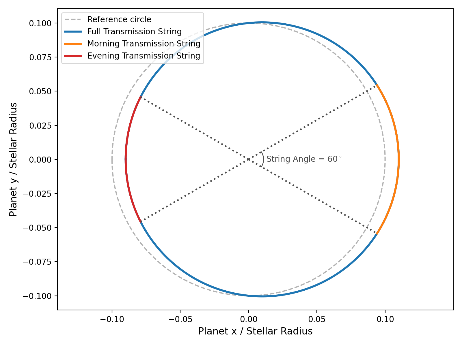
ncol
The number of columns you want in your LaTeX formatted tables. Defaults to 4.
star_Rad
The stellar radius. Used to compute the scale height if y_unit is transmission type and isplots_S6>=3.
planet_Teq
The planet’s zero-albedo, complete redistribution equlibrium temperature in Kelvin. Used to compute the scale height if y_unit is transmission type and isplots_S6>=3.
planet_Mass
The planet’s mass in units of Jupiter masses. Used to compute the scale height if y_unit is transmission type and isplots_S6>=3.
planet_Rad
The planet’s radius in units of Jupiter radii. Set to None to use the average fitted radius. Used to compute the scale height if y_unit is transmission type and isplots_S6>=3.
planet_mu
The mean molecular mass of the atmosphere (in atomic mass units). Used to compute the scale height if y_unit is transmission type and isplots_S6>=3.
planet_R0
The reference radius (in Jupiter radii) for the scale height measurement. Set to None to use the mean fitted radius. Used to compute the scale height if y_unit is transmission type and isplots_S6>=3.
isplots_S6
Sets how many plots should be saved when running Stage 6. A full description of these outputs is available here: Stage 6 Output.
hide_plots
If True, plots will automatically be closed rather than popping up on the screen.
topdir + inputdir
The path to the directory containing the Stage 5 JWST data. Directories containing spaces should be enclosed in quotation marks.
topdir + outputdir
The path to the directory in which to output the Stage 6 JWST data and plots. Directories containing spaces should be enclosed in quotation marks.
topdir + model_spectrum
The path to a model spectrum to plot underneath the observations to show how the fitted results compare to the input model for simulated observations or how the fitted results compare to a retrieved model for real observations. Set to None if no model should be plotted. The file should have column 1 as the wavelength and column 2 should contain the transmission or emission spectrum. Any headers must be preceded by a #. Directories containing spaces should be enclosed in quotation marks.
model_x_unit
The x-unit of the model. This can be any unit included in astropy.units.spectral (e.g. um, nm, Hz, etc.) but cannot include wavenumber units.
model_y_param
The y-unit of the model. Follow the same format as y_params. If desired, can be rp if y_params is rp^2, or vice-versa. Only one model model_y_param can be provided, but if y_params is a list then the code will only use model_y_param on the relevant plots (e.g. if model_y_param=rp, then the model would only be shown where y_params is rp or rp^2).
model_y_scalar
Indicate whether model y-values have already been scaled (e.g. write 1e6 if model_spectrum is already in ppm).
model_zorder
The zorder of the model on the plot (0 for beneath the data, 1 for above the data).
model_delimiter
Delimiter between columns. Typical options: None (for whitespace), ‘,’ for comma.