⚡️ Eureka! Quickstart ⚡️
Want to get up and running with Eureka!, but not really sure where to begin? Keep reading!
1. Installation 📦
The first thing you need to do is install the package, so if you haven’t already, take a break from this page and follow the Installation instructions (if you have issues be sure to visit the FAQ first).
2. Download the data 💾
With the installation complete, you’ll need some data to run Eureka! on. For now let’s use some simulated data that was produced for the Transiting Exoplanet Community ERS Data Challenge. Datasets for all four instruments are available on the STScI Box site, however, for the rest of this quickstart guide the NIRSpec Tiny dataset will be used.
Now, I’m sure you wouldn’t just leave the data in your Downloads folder, but if so, let’s make a new directory to store things instead. For example:
mkdir /User/Data/JWST-Sim/NIRSpec/
cd /User/Data/JWST-Sim/NIRSpec/
unzip -j ~/Downloads/Tiny.zip -d .
Note that for Eureka! you do not need to download any ancillary data - any additional files will be downloaded automatically (if you correctly set the CRDS environment variables during installation).
3. Set up your run directory 🗂
3.1 Gather the demo files
We’re almost there, but before you can get things running you need to set up a directory for Eureka! to store both input and output files.
mkdir /User/DataAnalysis/JWST/MyFirstEureka
cd /User/DataAnalysis/JWST/MyFirstEureka
From here, the simplest way to set up all of the Eureka input files is to download them from the JWST demos directory on the Github repository (direct download). Then we can copy them over:
mkdir demos
unzip -j ~/Downloads/JWST.zip -d ./demos
This demos directory contains a selection of template files to run Eureka!. There are three different types of files:
*.ecf: These areEureka!control files and contain input parameters required to run each stage of the pipeline. For more detail on the ecf parameters for each stage, see here.
*.epf: This is aEureka!parameter file and describes the initial guesses and priors to be used when performing light curve fitting (Stage 5).
run_eureka.py: A script to run theEureka!pipeline.
3.2 Customise the demo files
You might notice that not all of the demo files will be applicable to every dataset, either because they are tailored to a specific instrument, or because they are for a Eureka! pipeline stage that precedes the input data. This is the case for the NIRSpec data being used here, which as a *rateints.fits file (more information on JWST pipeline products here) has already been processed through an equivalent to Stage 1 of Eureka!.
So, let’s only copy over the specific files needed to process this NIRSpec dataset further. Given that the dataset contains a transit for WASP-39b, let’s also change some of the default filenames to something a little more informative:
cp demos/run_eureka.py .
cp demos/S2_nirspec_fs_template.ecf S2_wasp39b.ecf
cp demos/S3_nirspec_fs_template.ecf S3_wasp39b.ecf
cp demos/S4_template.ecf S4_wasp39b.ecf
cp demos/S5_template.ecf S5_wasp39b.ecf
cp demos/S5_fit_par_template.epf S5_fit_par_wasp39b.epf
cp demos/S6_template.ecf S6_wasp39b.ecf
Notice that all of the *.ecf files have a common wasp39b string. It’s useful to keep this homogenous across files as it is what Eureka! interprets as an “event label”, and is used to locate specific input files when running the pipeline. To see this more clearly, open up the run_eureka.py file and look at how the individual stages are being called. While you’re here, modify the eventlabel string directly to match the chosen naming:
eventlabel = 'wasp39b'
Finally, you need to connect everything together by opening up each .ecf file and updating the topdir, inputdir, and outputdir parameters within. For the S2_wasp39b.ecf, you want something like:
topdir          /User
inputdir        /Data/JWST-Sim/NIRSpec
outputdir       /DataAnalysis/JWST/MyFirstEureka/Stage2
However, for the later stages you can use something simpler, e.g. for the S3_wasp39b.ecf:
topdir          /User/DataAnalysis/JWST/MyFirstEureka
inputdir        /Stage2
outputdir       /Stage3
The explicit settings for the S4_wasp39b.ecf, S5_wasp39b.ecf and S6_wasp39b.ecf will be skipped here for brevity (but you should still do them!). However, it is important to notice a few settings in the S5_wasp39b.ecf. Specifically, you need to assign the correct .epf file, and modify the number of processors you want to use during the light curve fitting.
ncpu            4
fit_par         S5_fit_par_wasp39b.epf
To speed up the Stage 5 dynesty fit, you can also reduce the number of live points (run_nlive) at the cost of a more coarse corner plot in the end. The bare minimum recommended value is
ndim * (ndim + 1) / 2
and our fit presently has ndim=10 free values in the EPF, so that means a bare minimum of 55 live points. As a compromise, let’s use 256 live points instead to
get a fairly nice corner plot but also speed up the fit, so set the following in S5_fit_par_wasp39b.epf:
run_nlive 256
While editing all those files, you may have noticed that there is a whole range of other inputs that can be tweaked and adjusted at each different stage. For now you can ignore these as the demo files have been specifically tailored to this simulated dataset of WASP-39b.
4. Run Eureka! 💡
Now that everything is set up, you should now be able to run the pipeline using:
python run_eureka.py
This will start printing information to your terminal, saving a bunch of output data/figures to the outputdir file locations you assigned above, and depending on the number of processors you were brave enough to allocate, potentially make your laptop as noisy as the engine of a Boeing 747.
Carry on reading for more information on each individual stage in the pipeline and some of the products it produces. Alternatively, feel free to dig through the output directories and get a gauge of what each stage is doing at your own speed.
Stage 1: Ramp Fitting
Stage 1 takes individual ramp level images and collapses them into integration level images, alongside some other basic corrections. This Stage broadly follows the STScI JWST pipeline methodology, with a few opportunities for adjustment as detailed on the .ecf information page.
The NIRSpec data being used here has already undergone the equivalent of this Stage, and it is therefore skipped (you will also notice it is commented out in the run_eureka.py file).
Stage 2: Calibrations
Stage 2 calibrates the data by performing a range of steps such as flat fielding and photometric unit conversions. Similarly to Stage 1, this broadly follows the STScI JWST pipeline methodology. In the case of the NIRSpec dataset we are using, the Eureka! implementation of this Stage avoids any spatial trimming of the images that usually occurs with the STScI pipeline. This facilitates a more accurate correction of the background and 1/f noise during Stage 3, as more background pixels are retained.
Stage 3: Reduction
From Stage 3 onwards, Eureka! no longer makes use of the STScI pipeline and instead implements a range of custom routines to reduce the data further. It’s at this stage that background subtraction and spectral extraction is performed, resulting in 1D spectra that can be used for light curve analysis and fitting.
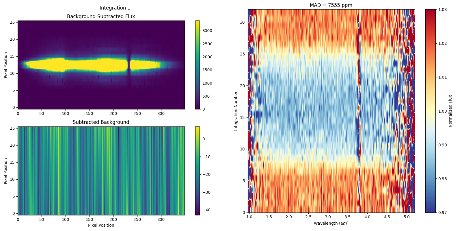
By entering the figs folder you’ll find a range of diagnostic figures. For example, on the left hand side of the figure copied below, the background subtracted 2D spectrum for the first integration is plotted (top) alongside a 2D image of the estimated background. Note that the distinct striping is a result of 1/f noise in the NIRSpec detector electronics, and is dominant along pixel columns as they correspond to the direction of the detector readout.
To the right you can see a 2D representation of the variation in flux between consecutive integrations as a function of wavelength. In fact, the transit of WASP-39b can be seen via the horizontal band of reduced flux between integrations ~9-25. At the top, the median absolute deviation (MAD) for the entire dataset is displayed, and is calculated by determining the flux difference between each image and the next, for each wavelength, followed by taking the overall median of these values across all wavelengths and all images.
Finally, note that the actual data for these produced 1D spectra are contained in the *Table_Save.txt file.
Stage 4: Create Lightcurves
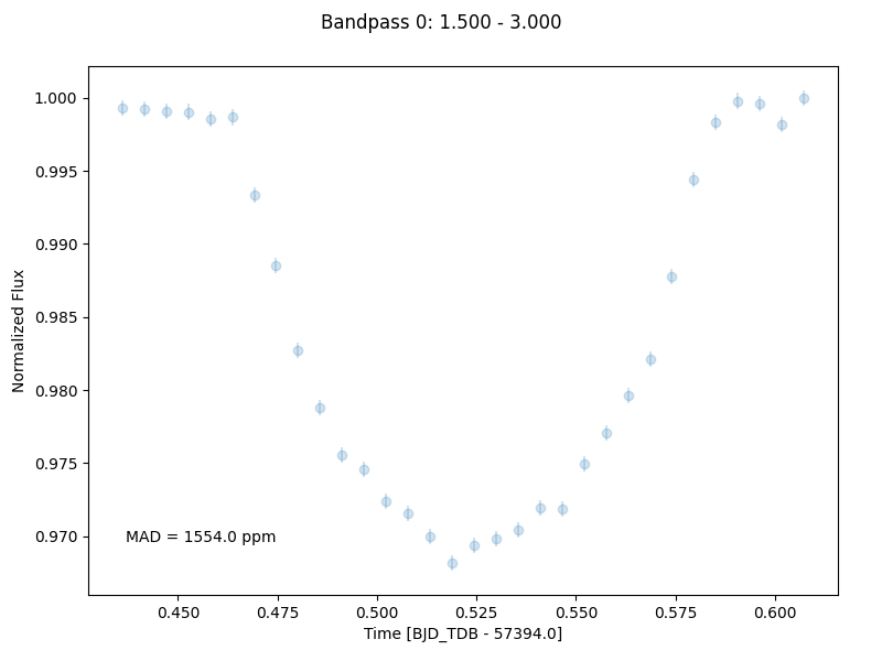
Stage 4 takes the 1D spectra produced by the previous stage and turns them in to light curves. The number of wavelength channels to turn into light curves, along with the wavelength range across which they will be calculated, can be defined in the Stage 4 .ecf file. In the interest of reducing the computational burden of the following light curve fitting stage, only two light curves will be generated corresponding to 1.5-3.0 μm and 3.0-4.5 μm (see figure below).
Similarly to Stage 3, the actual data for the produced light curves can be found in the *Table_Save.txt file.
Stage 5: Lightcurve Fitting
Stage 5 takes all of the lightcurves produced by the previous stage and performs a variety of fitting routines to estimate specific system and planetary properties. For this quickstart, the fitting was performed using nested sampling as implemented by dynesty, for a model assuming a transit of WASP-39b plus an aribitrary linear polynomial trend.
As a reminder, the input initial guesses and priors for the model properties are contained within the Stage 5 .epf file. To facilitate this quickstart demo, input parameters applicable to WASP-39b have already been assigned. For your own reductions, you’ll need to tailor this file to the system you are observing and the type of fit you want to perform.
We have used nested sampling during this quickstart, however, this is not the only fitting method - both a simple least-squares minimisation as implemented by scipy and a full MCMC as implemented by emcee can also be used. Given the computational demands of running nested sampling or MCMC, it’s advised that you perform initial testing with the least-squares fitter, before moving to a more advanced fitter. As the quickstart Stage 5 .ecf and .epf have already been prepared with suitable input values, we have skipped straight to a nested-sampling fit.
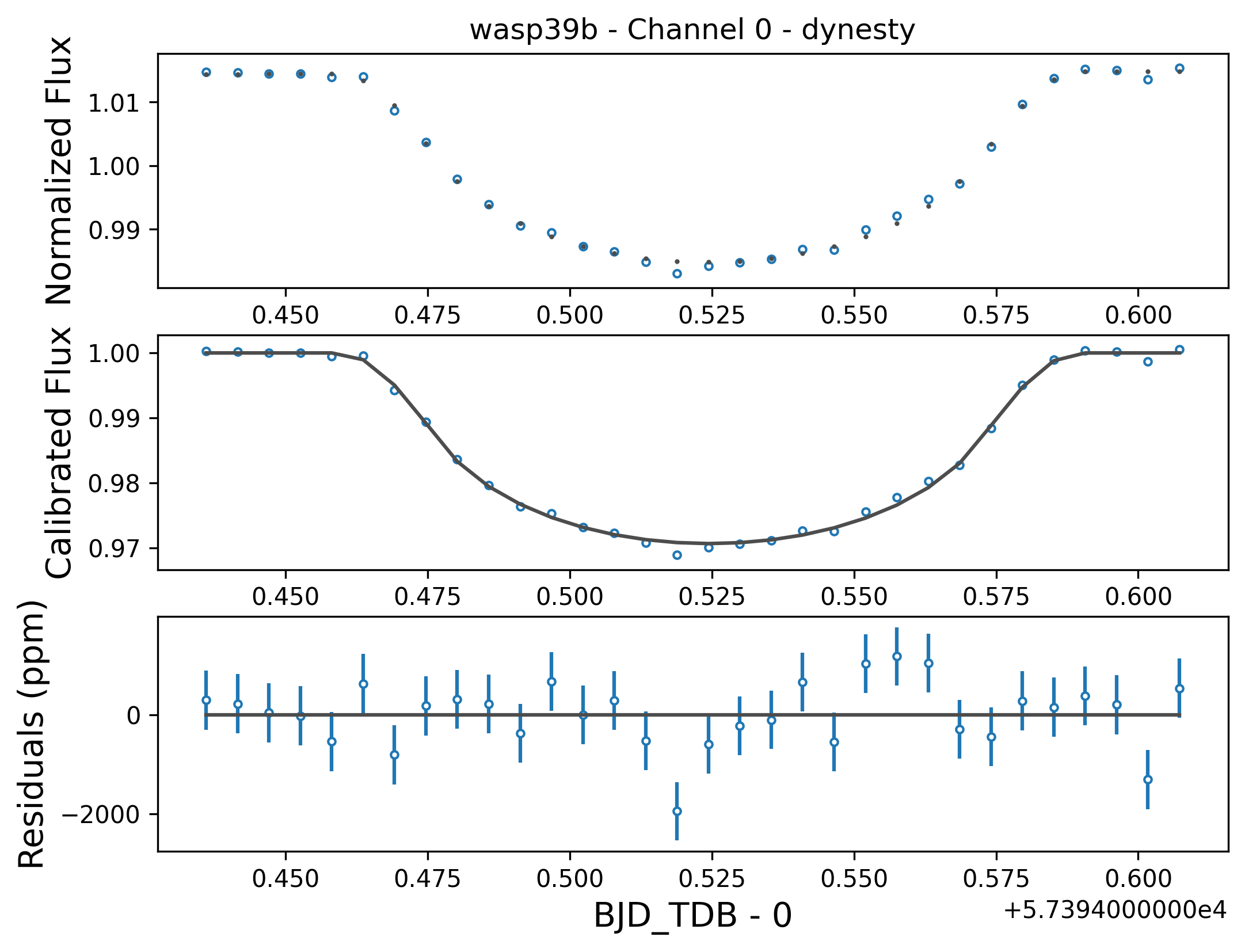
An example figure demonstrating the best fit model lightcurve alongside the data is shown below, and corner plot representations of the fit posteriors can be found under the figs directory. Once again, the actual model light curve data can be found in the *Table_Save_ch*.txt files.
Stage 6: Plot Spectra
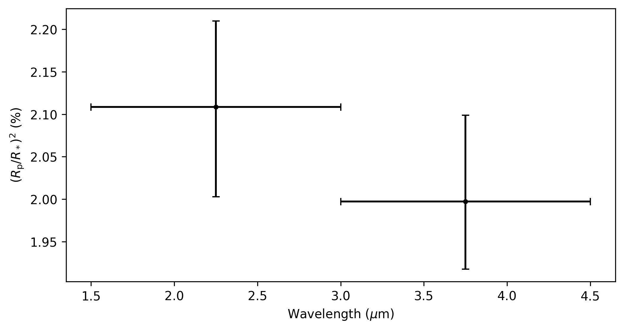
The final Stage of Eureka!, Stage 6, takes the output data from the lightcurve fitting and produces transmission and/or emission spectra. As mentioned earlier, this quickstart only makes use of two different light curves from this dataset from 1.5-3.0 μm and 3.0-4.5 μm. In this case, our transmission spectrum for the transit of WASP-39b will only have two data points (see figure below). Note that the errors bars are not representative of what could be expected for true JWST data, as to reduce the computational burden this dataset has been trimmed down from 8192 integrations to only 32. Finally, the transmission spectrum data is saved in the *Table_Save.txt file.
5. Where to go next 👩💻
You made it! Congratulations, it’s time to reward yourself with a break 😊
However, if this quickstart guide wasn’t enough to sate your appetite, consider taking a look at the different parameter settings within the *.ecf files here and tweak away! If you want to explore the NIRSpec Tiny Dataset further, head back to the Stage 4 .ecf and try increasing the number of wavelength channels. Once you’re comfortable, consider running things through with the full dataset. Or, if you’re bored with NIRSpec, maybe take a look at a simulated dataset for NIRCam, NIRISS, or MIRI instead.
If any bugs / errors cropped up while you were working through this quickstart, or if they turn up in the future, take a look at our FAQ or report an issue on our GitHub repository. Thanks!