Eureka! Outputs

Stage 2 through Stage 6 of Eureka! can be configured to output plots of the pipeline’s interim results as well as the data required to run further stages.

Stage 2 Outputs

If skip_extract_1d is set in the Stage 2 ECF, the 1-dimensional spectrum will not be extracted, and no plots will be made. Otherwise, Stage 2 will extract the 1-dimensional spectrum from the calibrated images, and will plot the spectrum.

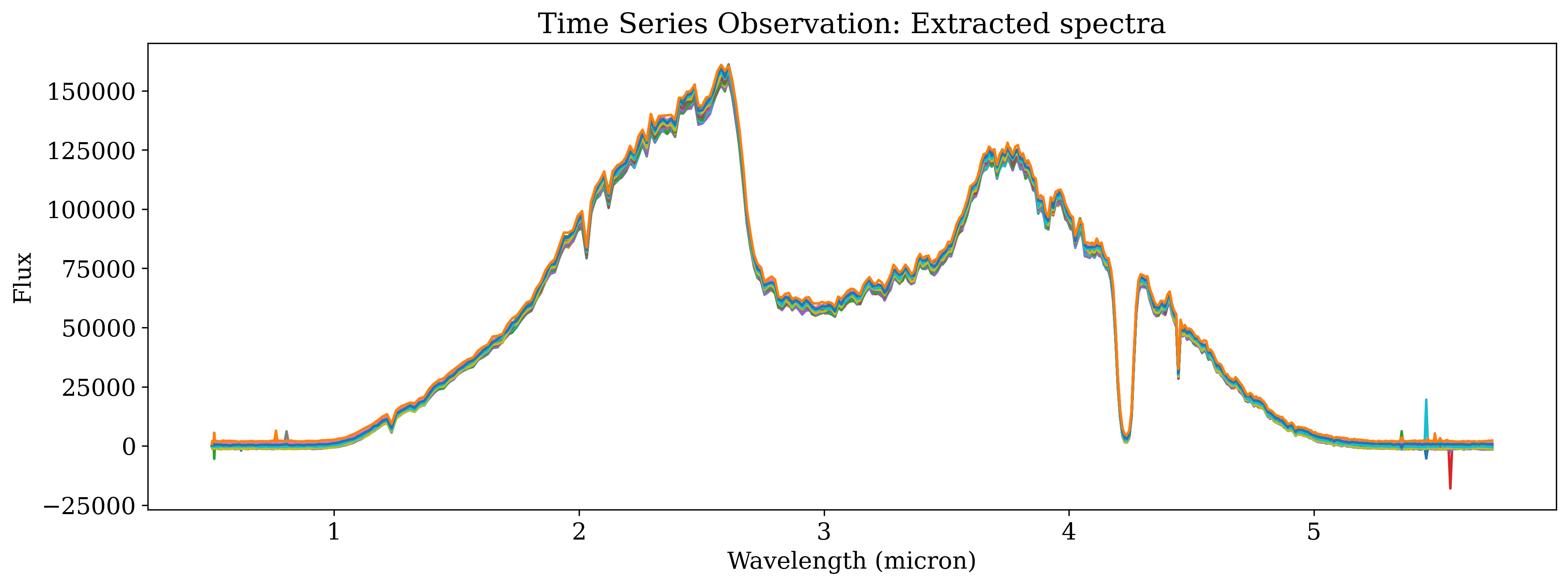
Fig 2101: 1-Dimensional Spectrum Plot

Stage 3 Outputs

In Stage 3 through Stage 5, output plots are controlled with the isplots_SX parameter. The resulting plots are cumulative: setting isplots_S3 = 5 will also create the plots specified in isplots_S3 = 3 and isplots_S3 = 1.

In Stage 3:

• If isplots_S3 = 1: Eureka! will plot the 2-dimensional, non-drift-corrected light curve, as well as variations in the source position and width on the detector.

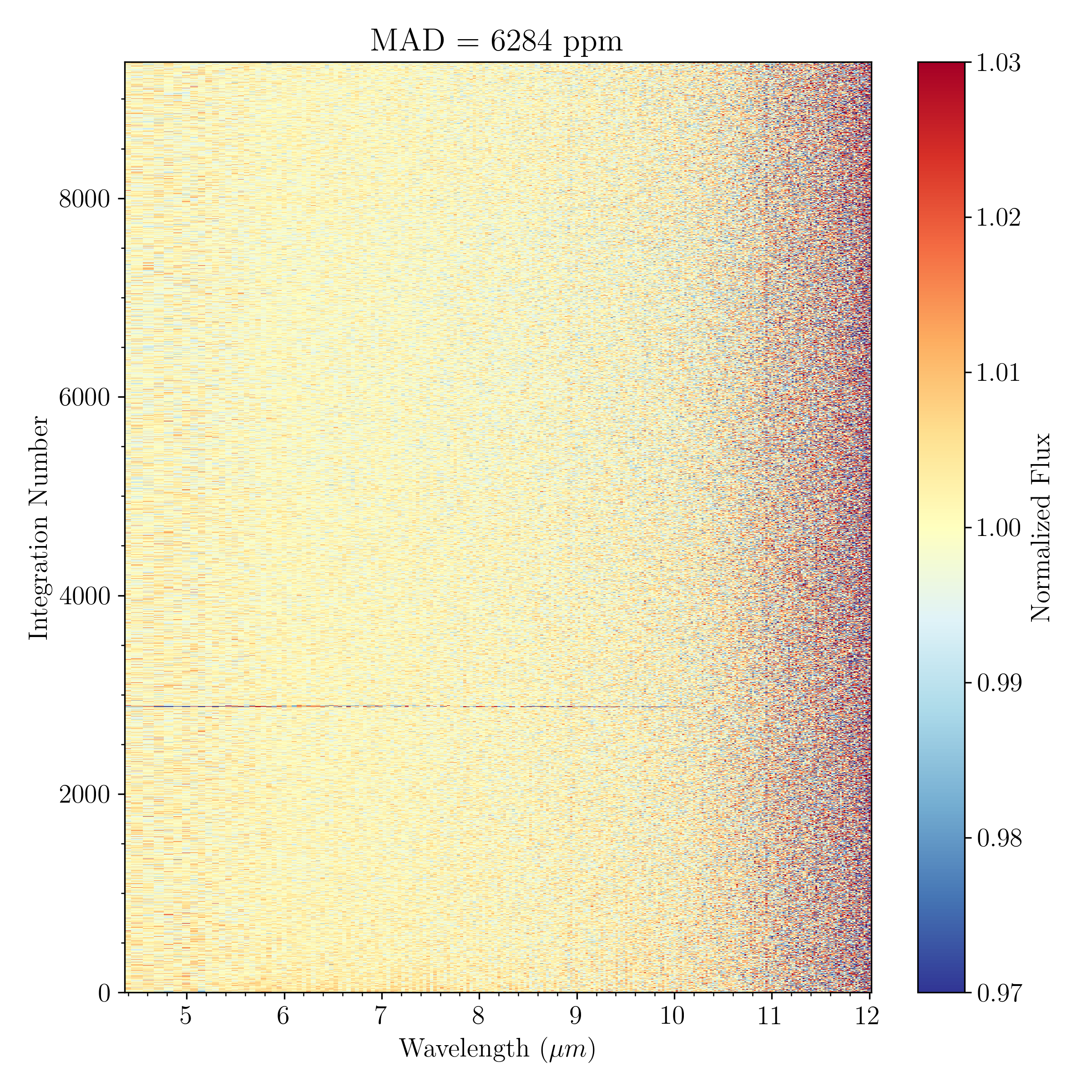
Fig 3101: 2-Dimensional Spectrum Plot with a linear wavelength x-axis

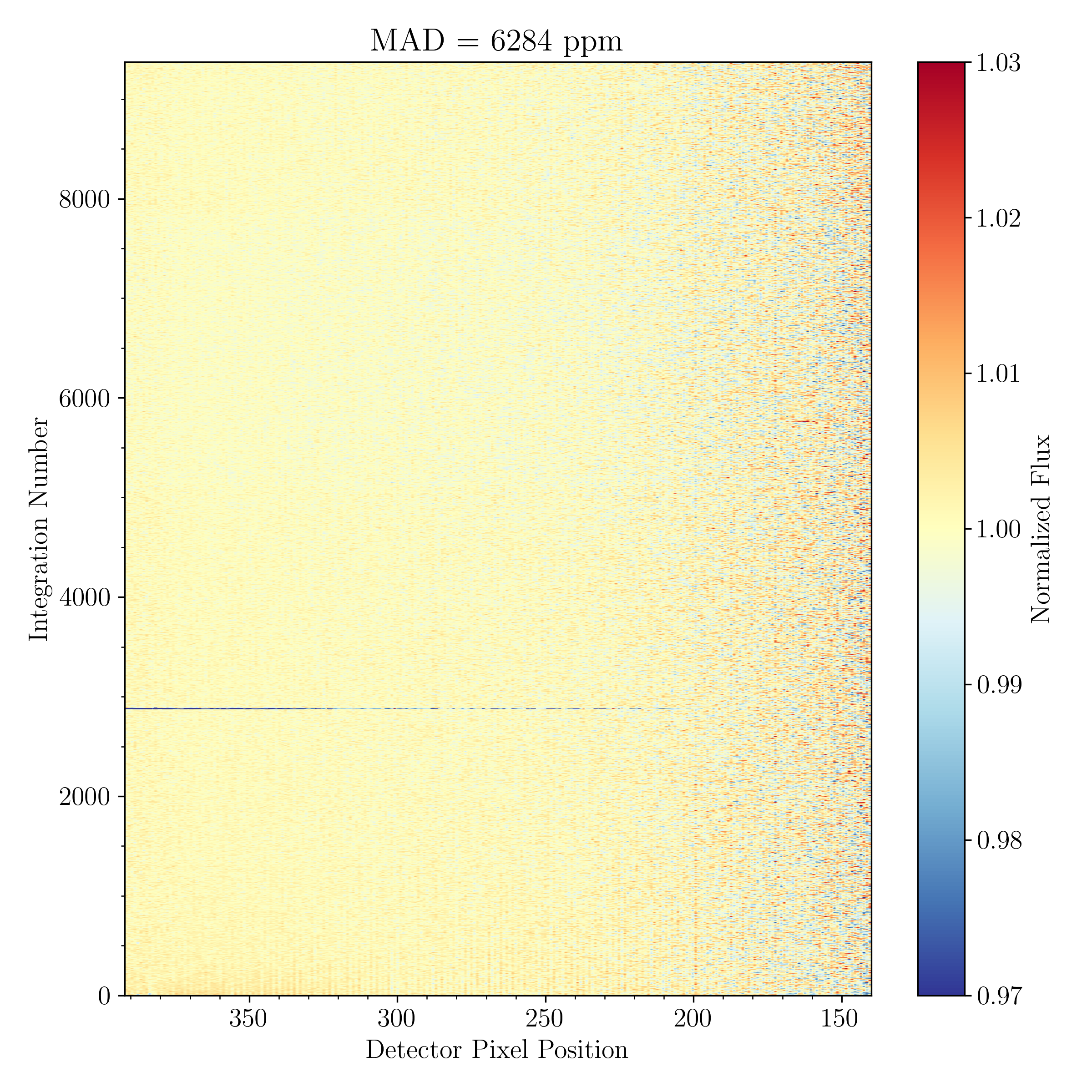
Fig 3102: 2-Dimensional Spectrum Plot with a linear detector pixel x-axis

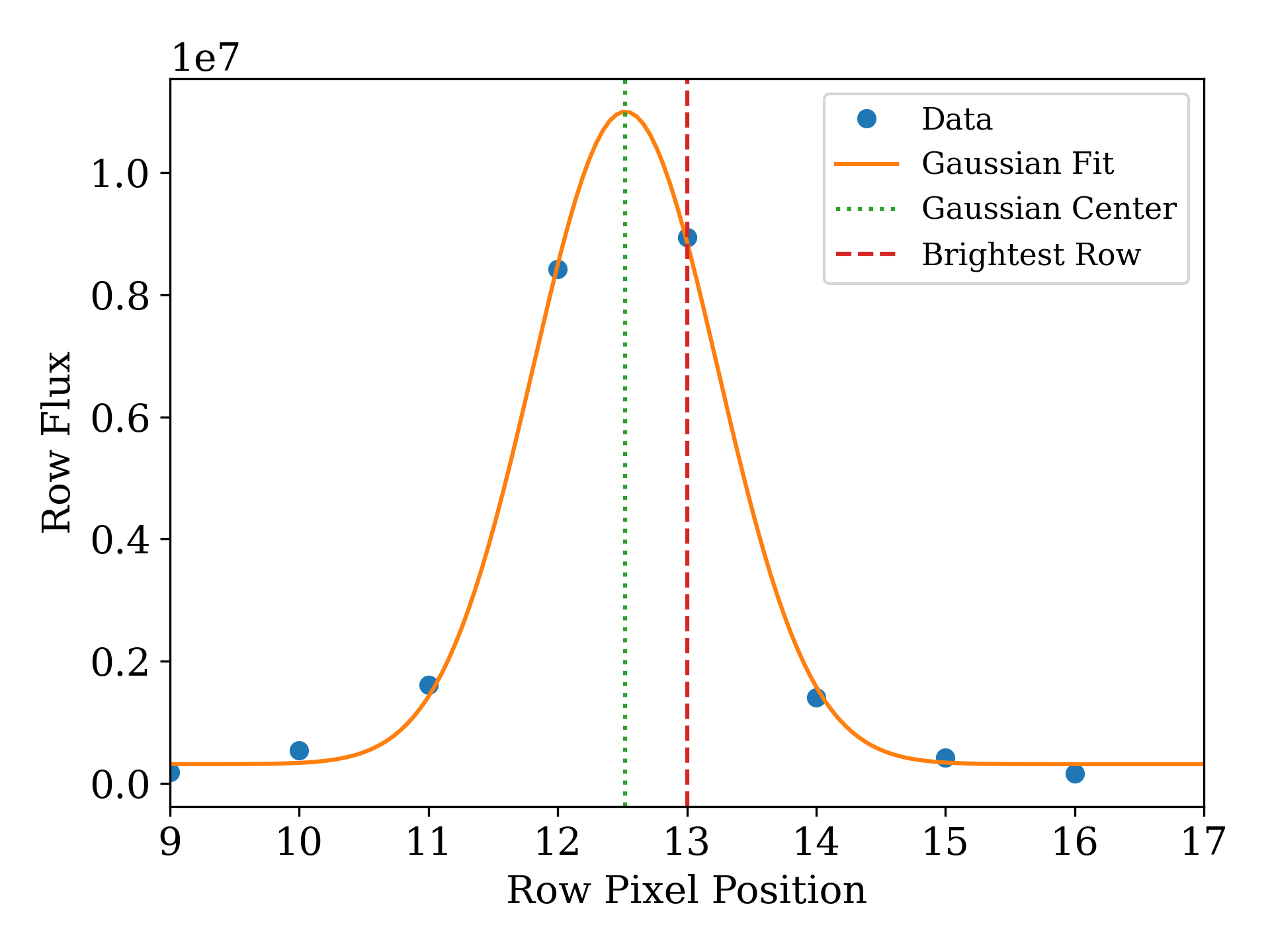
Fig 3103: Source Position Fit Plot

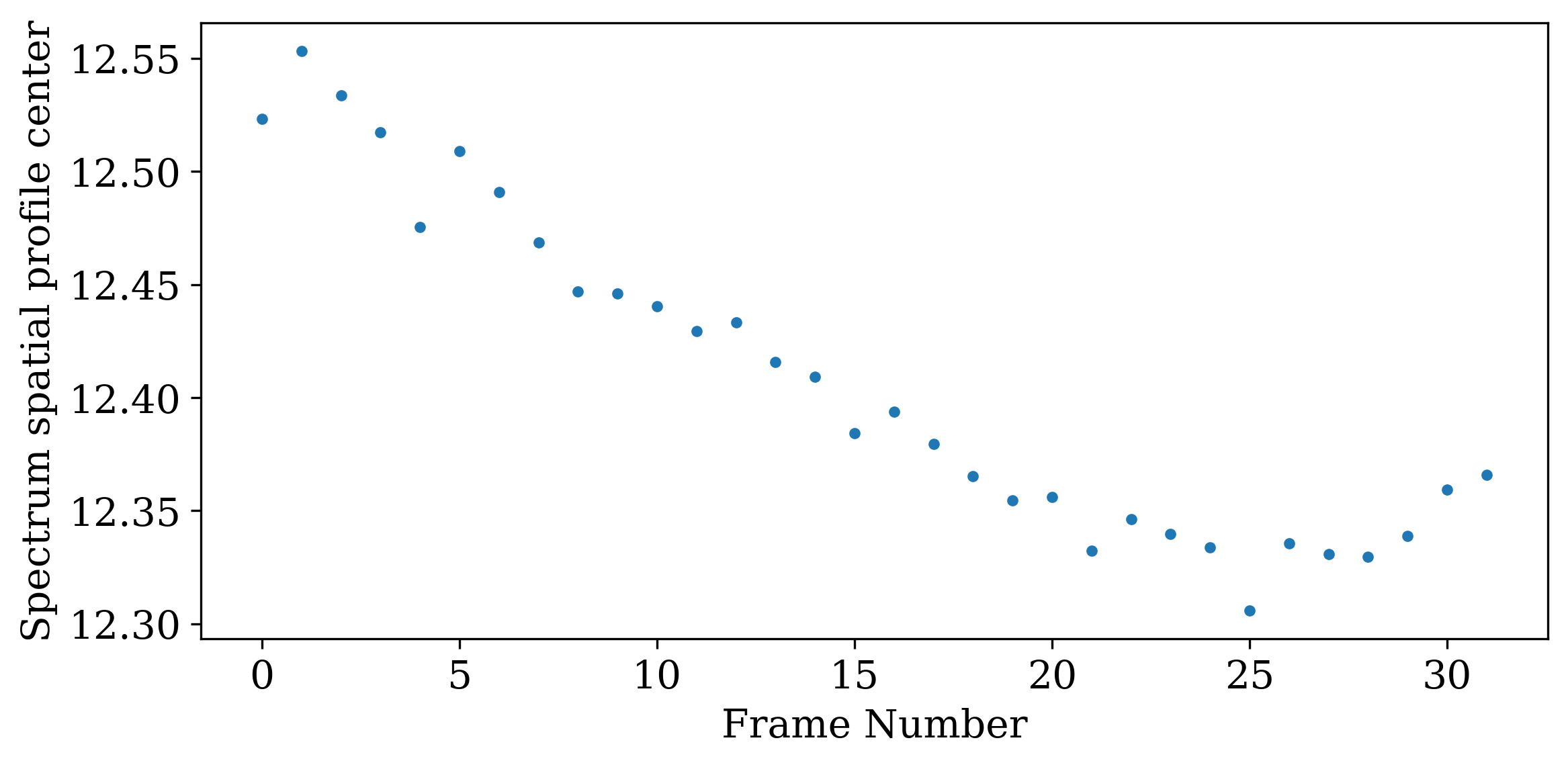
Fig 3104: Variations in the spatial-axis position

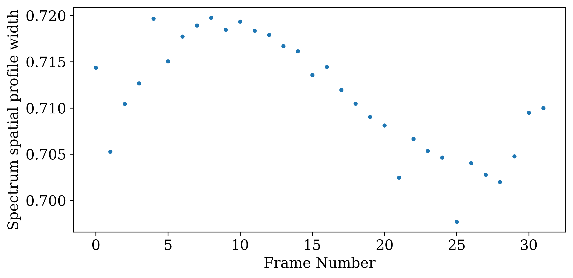
Fig 3105: Variations in the spatial-axis PSF width

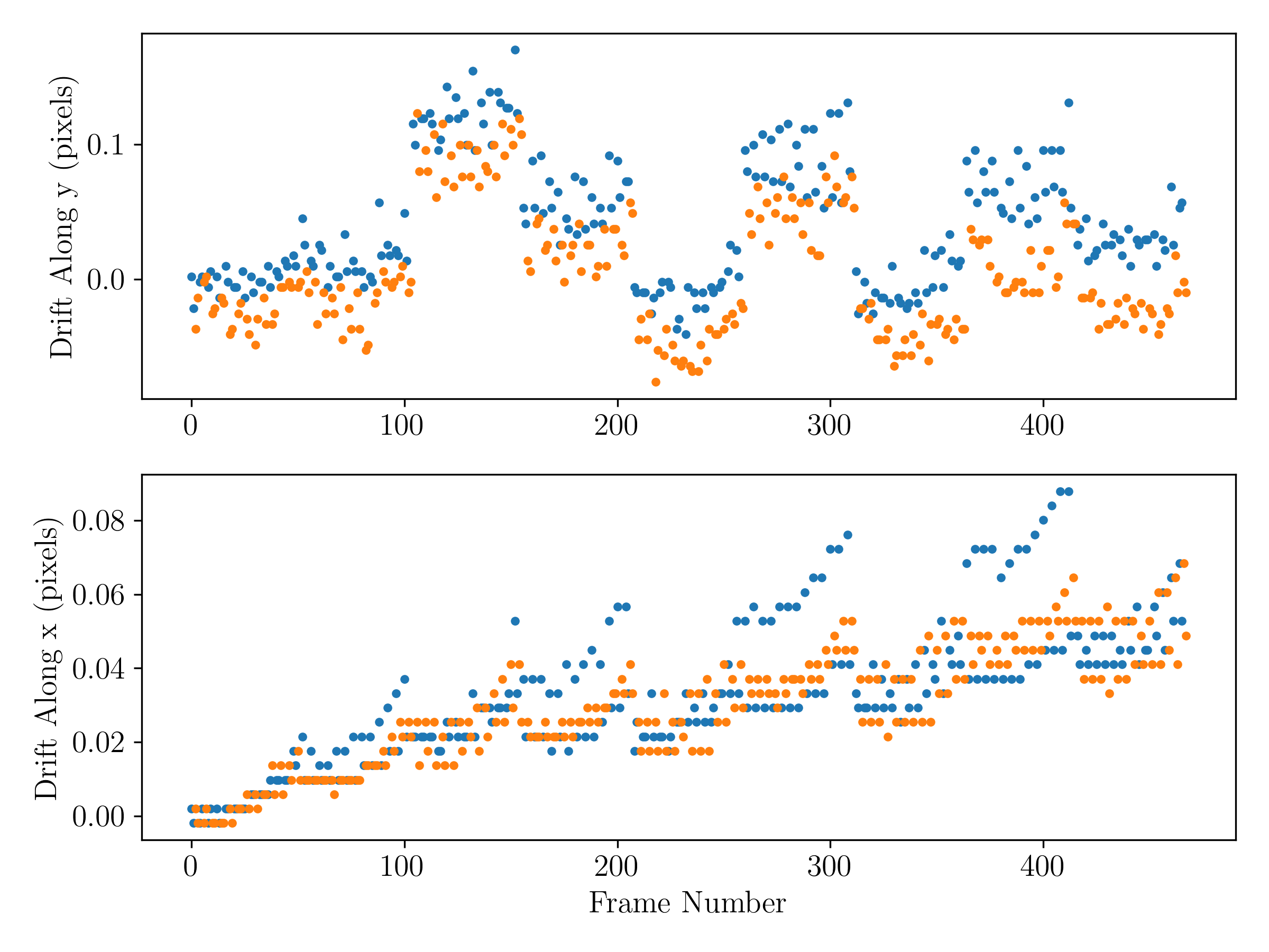
Fig 3106: 2D drift fit (currently only produced for WFC3)

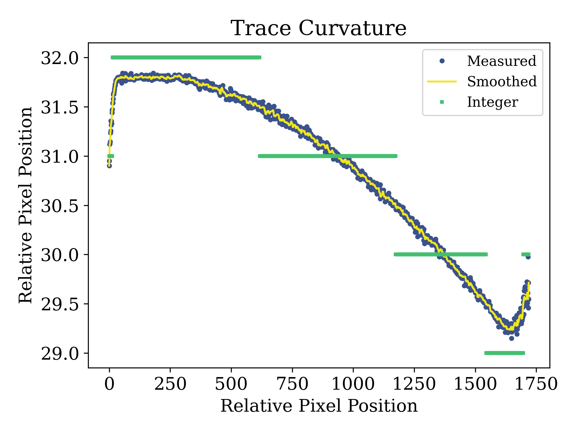
Fig 3107: Measured, smoothed, and integer-rounded position of trace

• If isplots_S3 = 3: Eureka! will plot the results of the background and optimal spectral extraction steps for each exposure in the observation as well as the cleaned median frame.

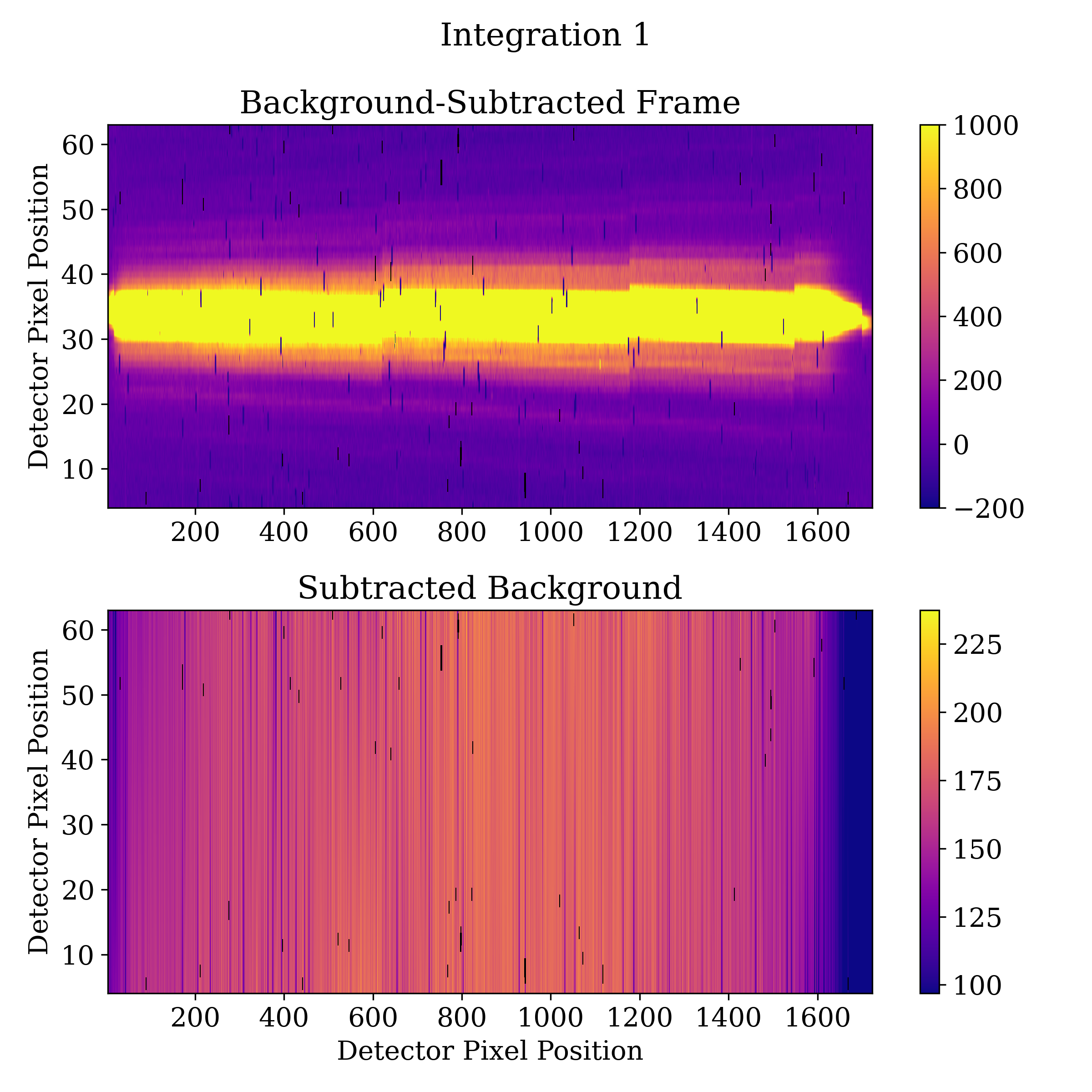
Fig 3301: Background Subtracted Flux Plot

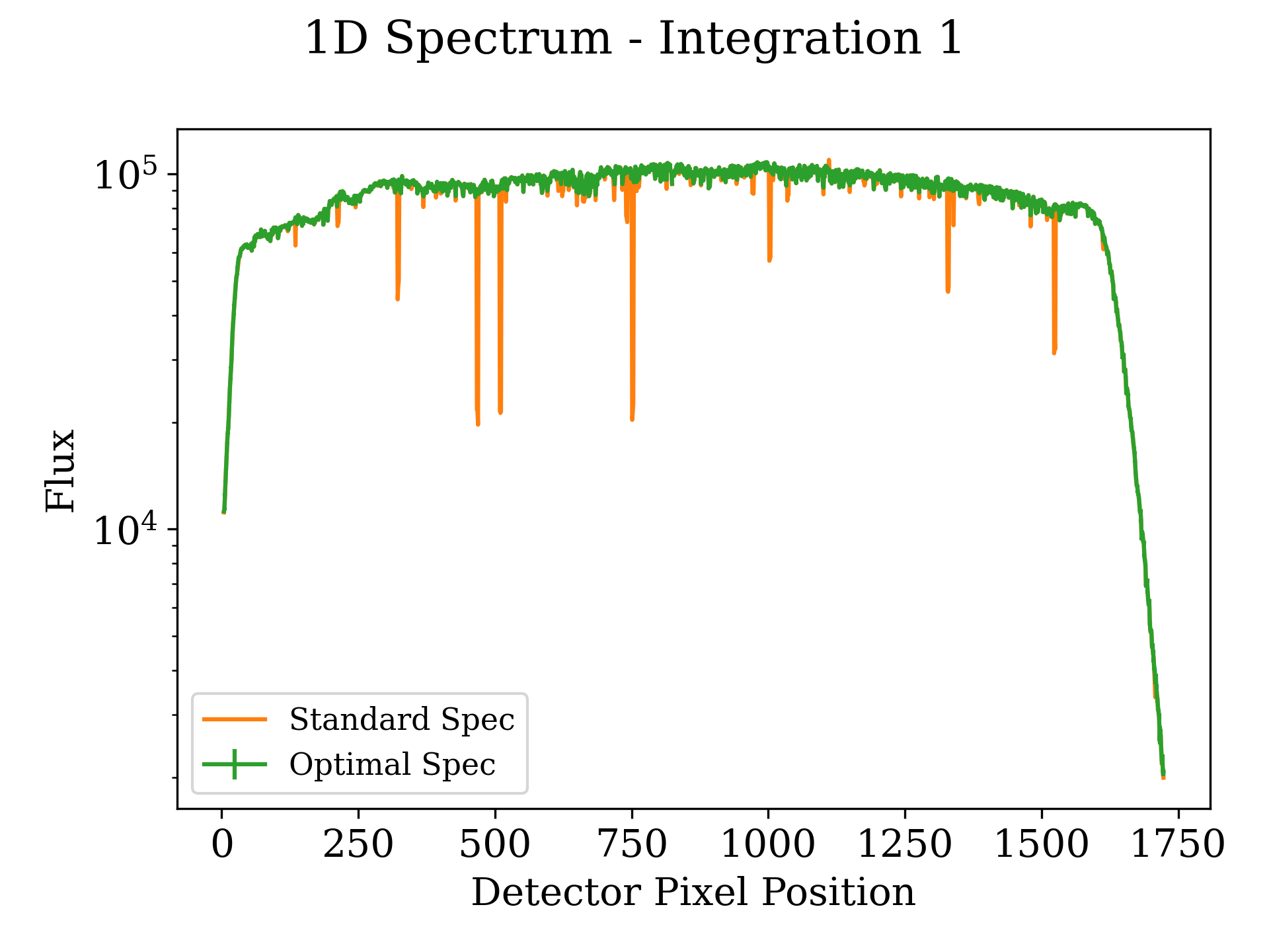
Fig 3302: 1-Dimensional Spectrum Plot

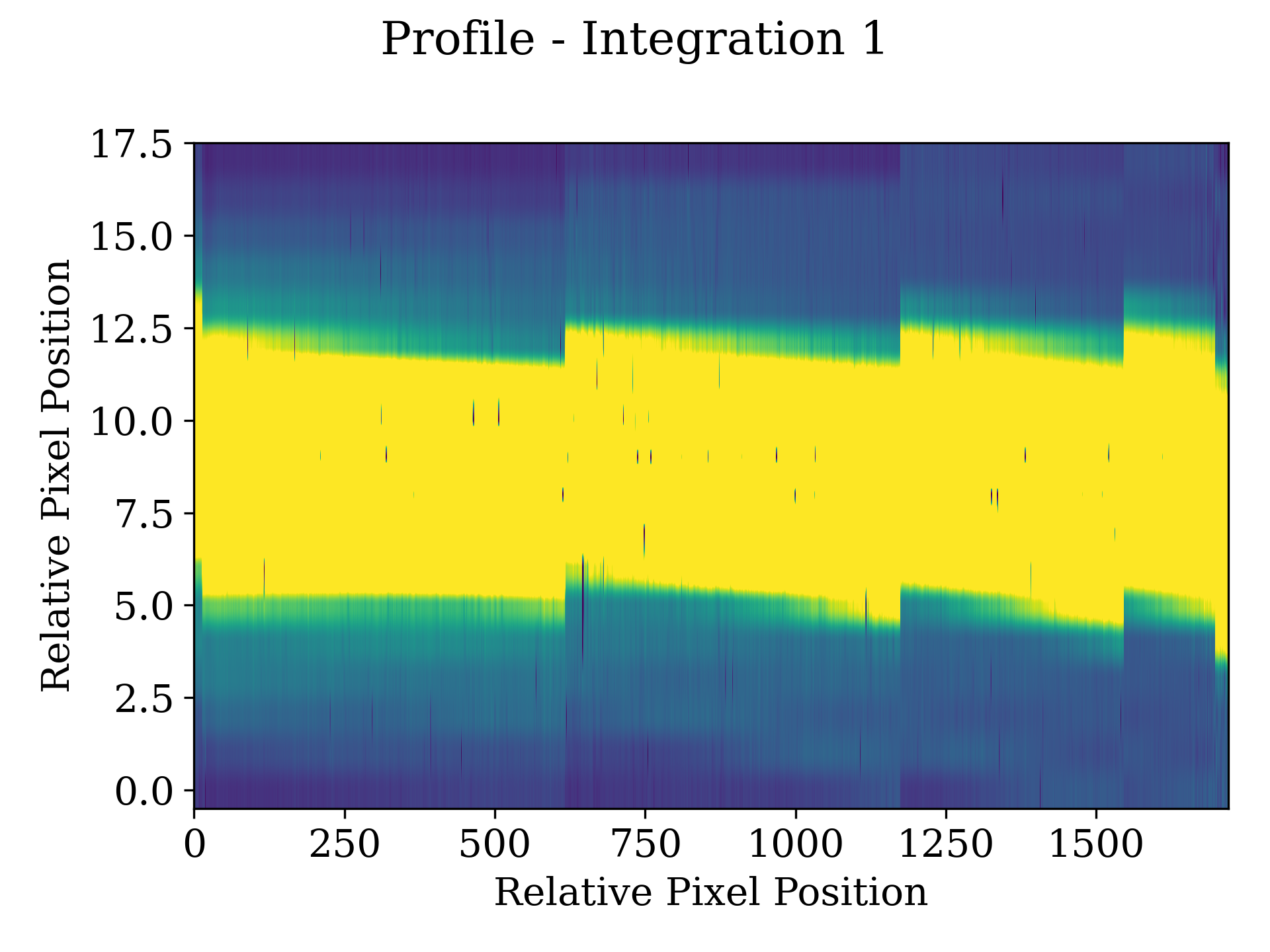
Fig 3303: Weighting Profile Plot

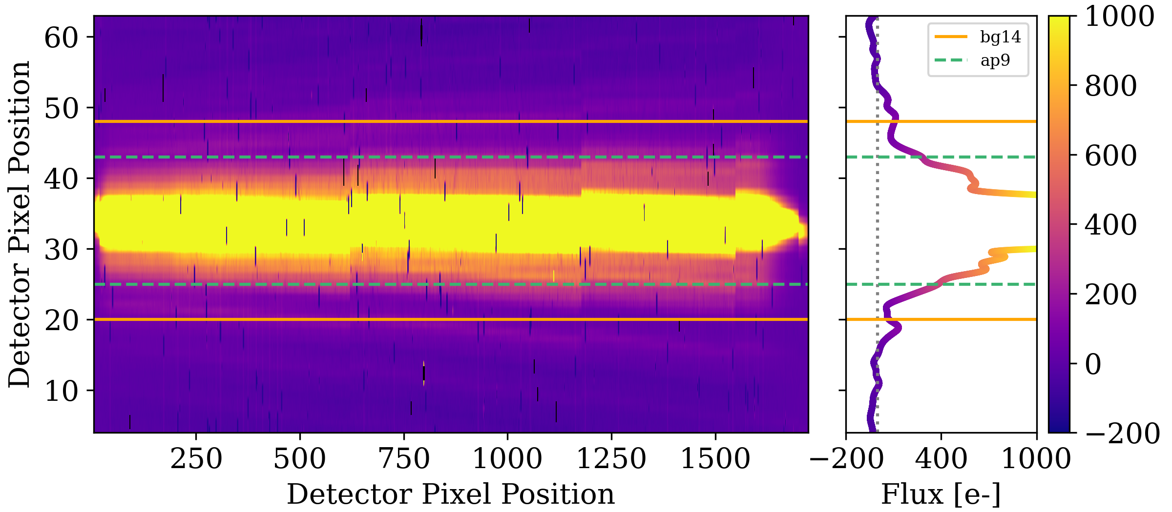
Fig 3304: Residual Background Plot

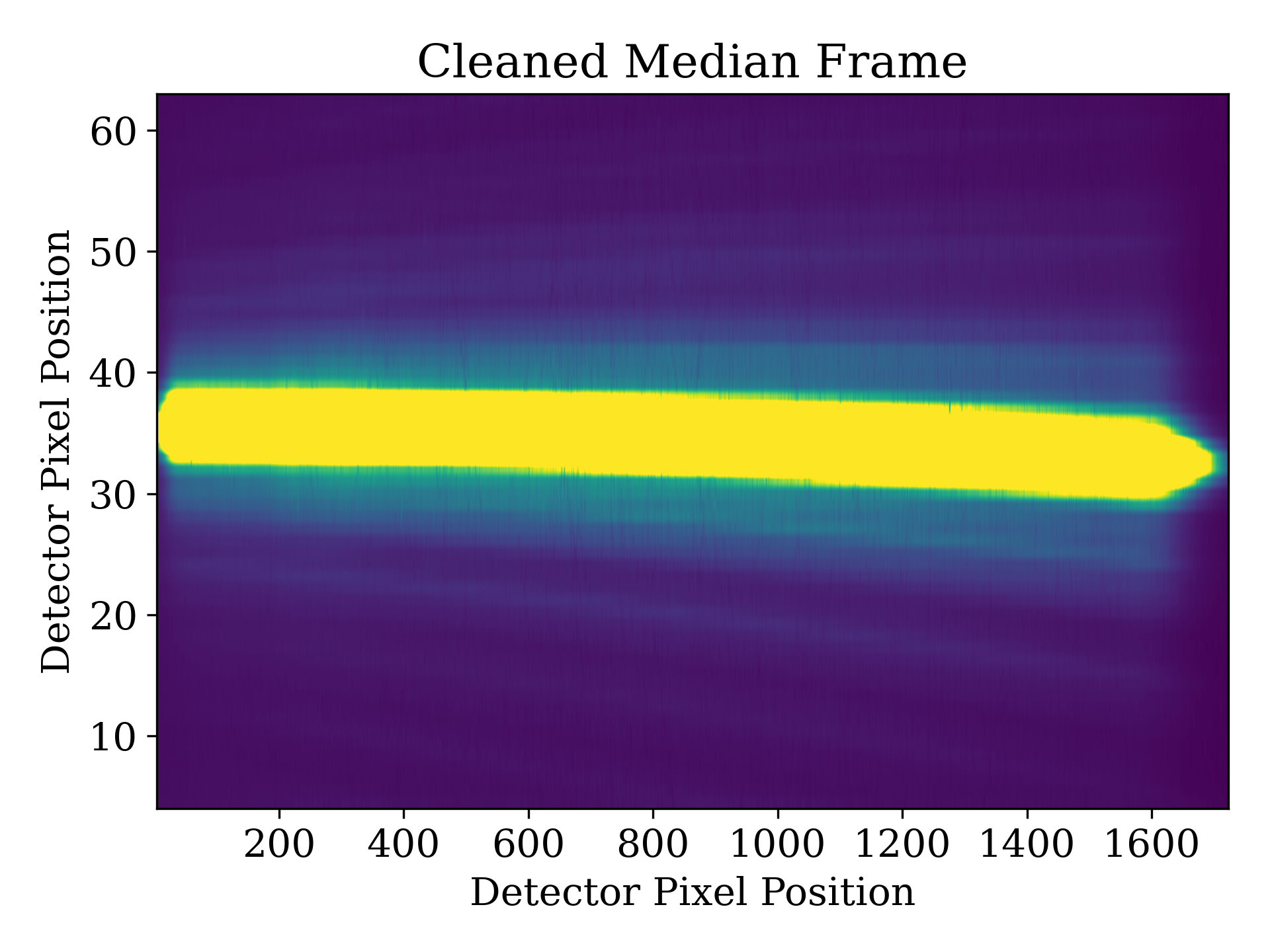
Fig 3308: Clean Median Frame Plot

• If isplots_S3 = 5: Eureka! will plot the Subdata plots from the optimal spectral extraction step.

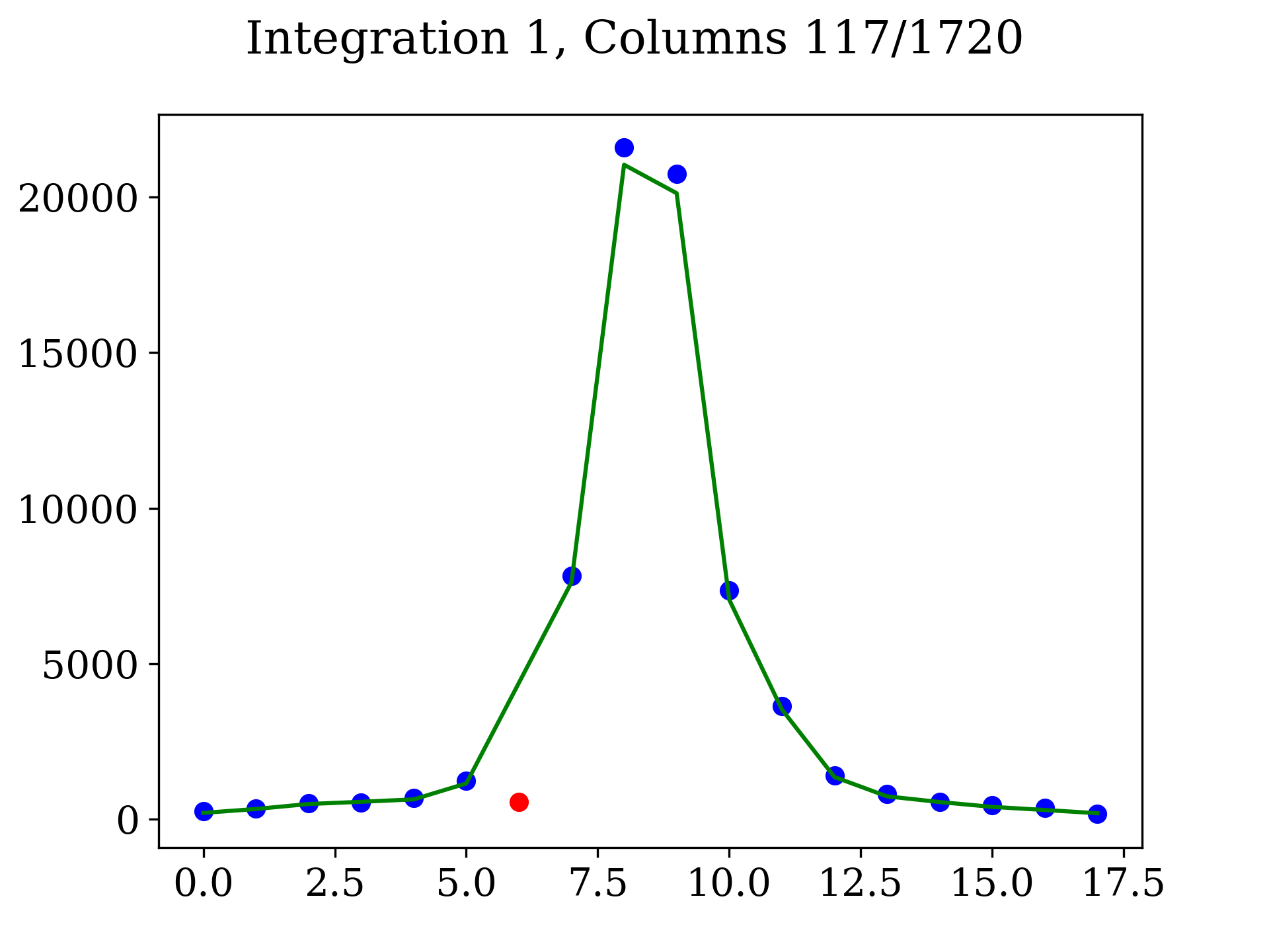
Fig 3501: Spectral Extraction Subdata Plot

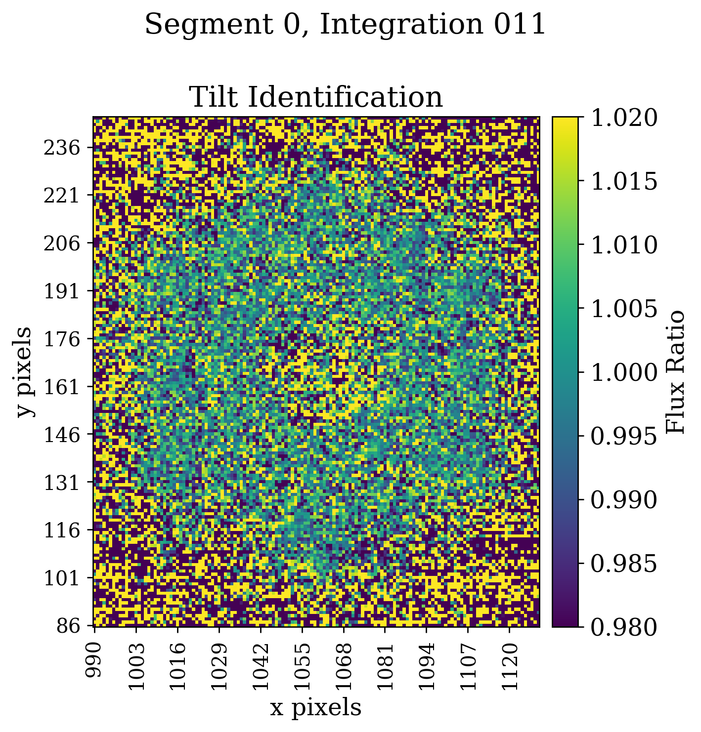
Fig 3507a: Tilt event frame plot. Figures 3507b and 3507c are GIF versions of this figure, b is at the segment level and c is over all segments

Stage 4 Outputs

In Stage 4:

• If isplots_S4 = 1: Eureka! will plot the spectral drift per exposure, the drift-corrected 2-dimensional lightcurve with extracted bins overlaid, and the 1D light curves.

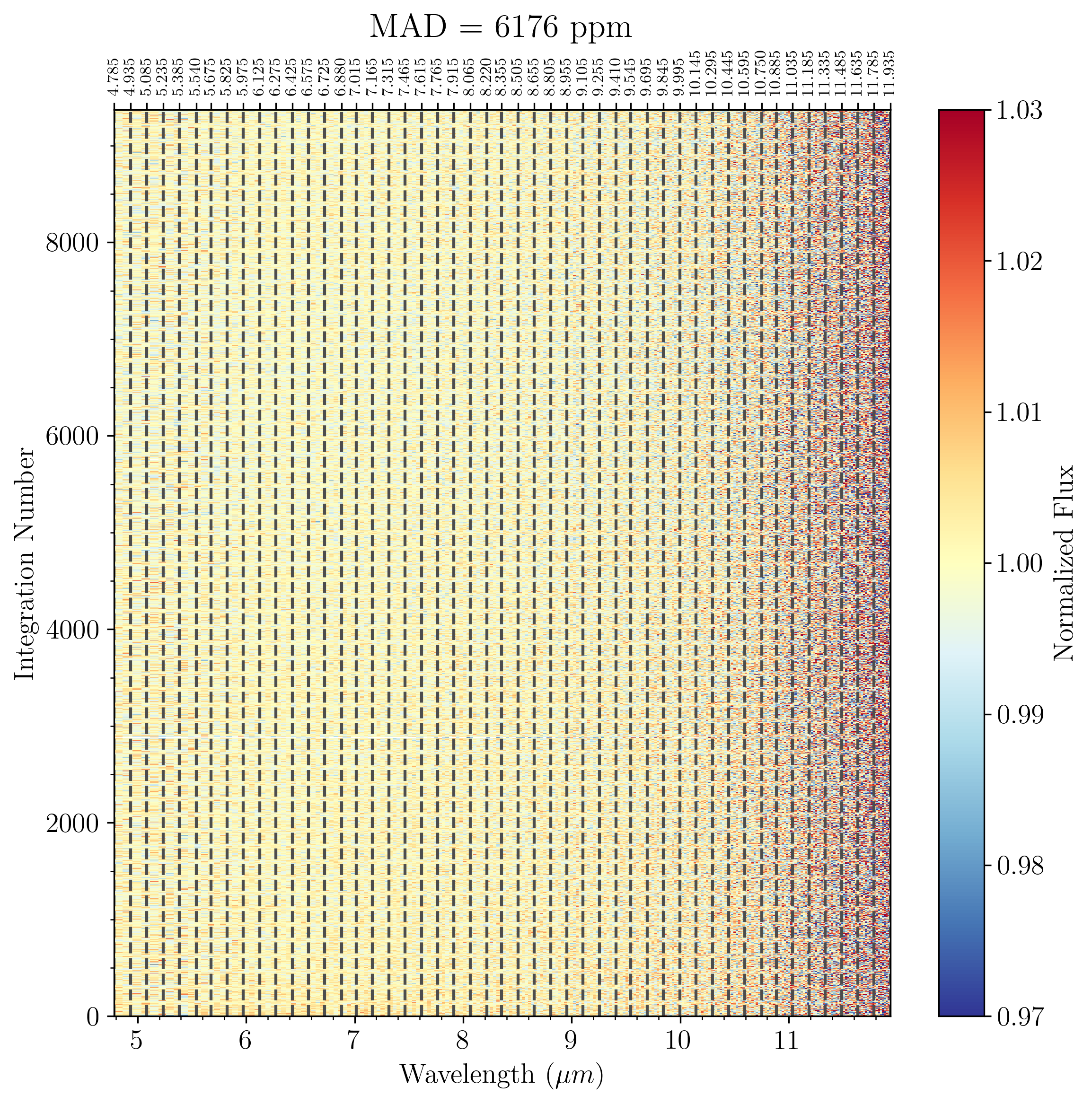
Fig 4101: 2-Dimensional Spectrum with a linear wavelength x-axis.

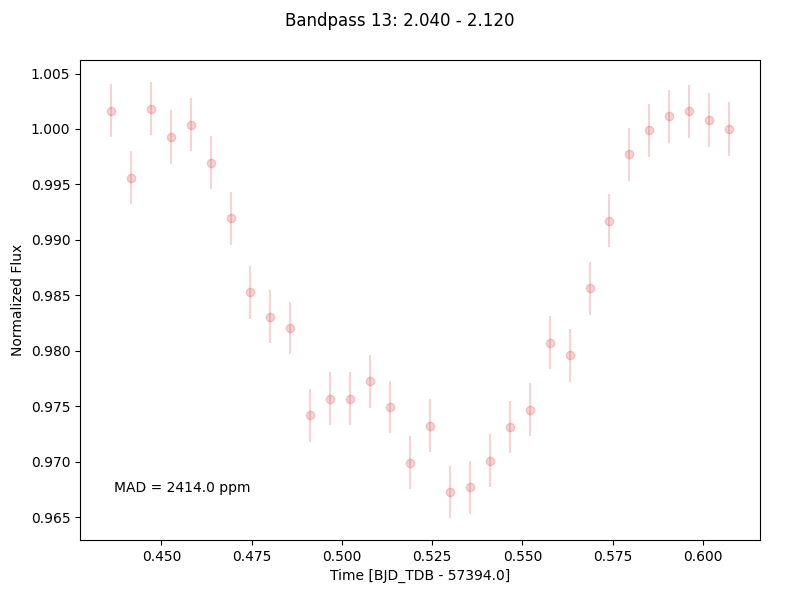
Fig 4102: 1-Dimensional Binned Spectrum

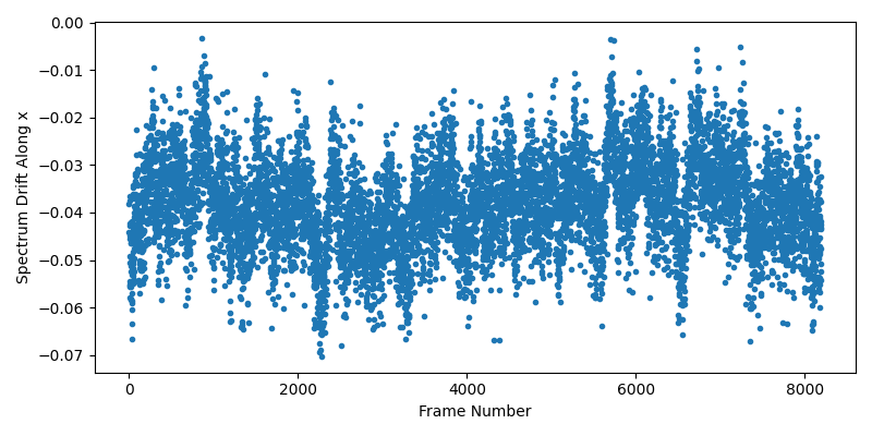
Fig 4103: Spectral Drift Plot

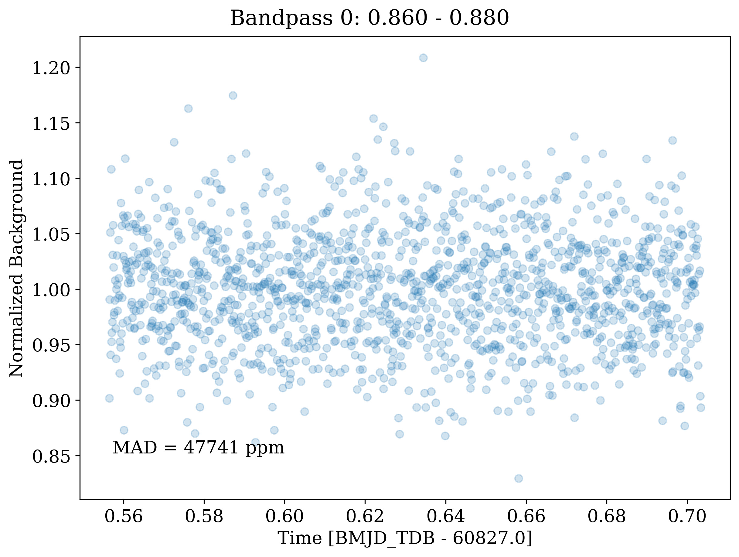
Fig 4105: Background Flux Plot

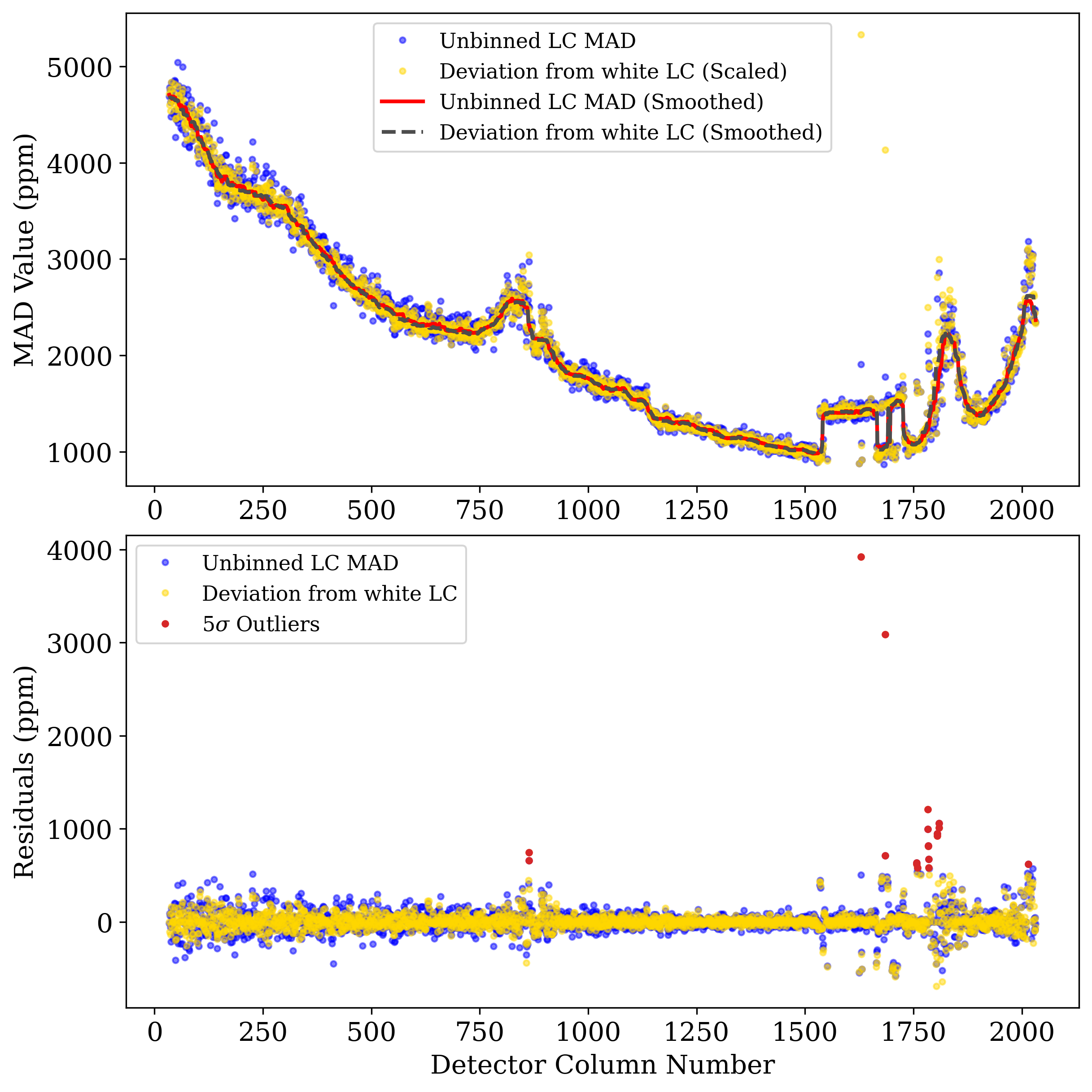
Fig 4106: MAD Outliers Plot

• If isplots_S4 = 3: Eureka! will plot the cross-correlated reference spectrum with the current spectrum for each integration, and the cross-correlation strength for each integration.

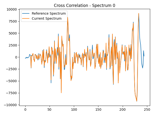
Fig 4301: Cross-Correlated Reference Spectrum

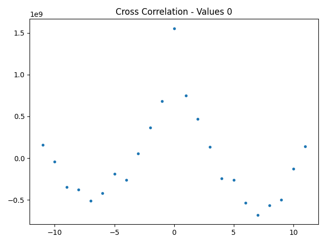
Fig 4302: Cross-Correlation Strength

Stage 5 Outputs

In Stage 5:

• If isplots_S5 = 1: Eureka! will plot the fitted lightcurve model over the data in each channel. If fitting with a GP, an additional figure will be made showing the GP component. If fitting a sinusoid_pc model, another zoomed-in figure with binned data will be made to emphasize the phase variations. Finally, an additional plot compares the fits from different fitters.

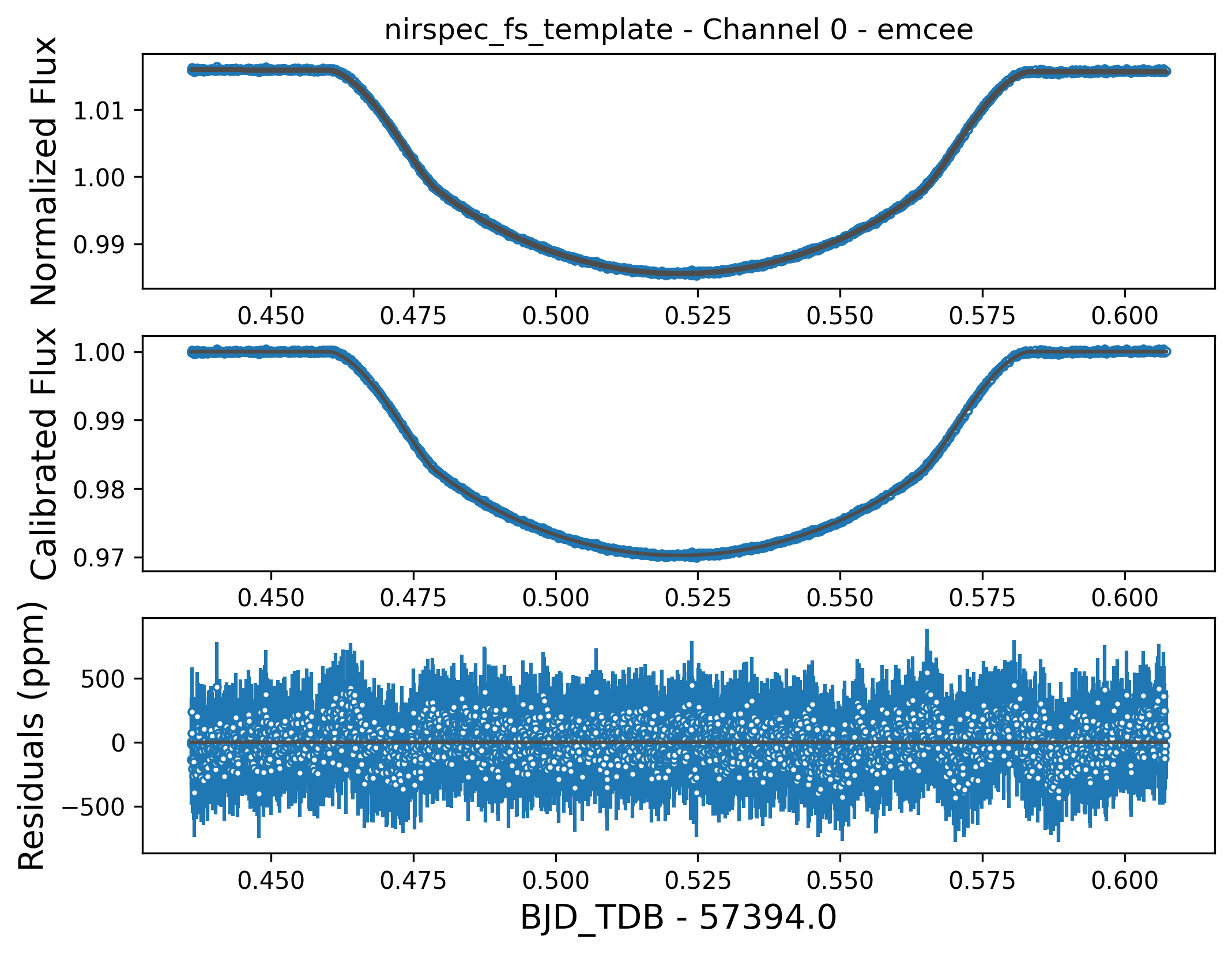
Fig 5101: Fitted Lightcurve, Model, and Residual Plot

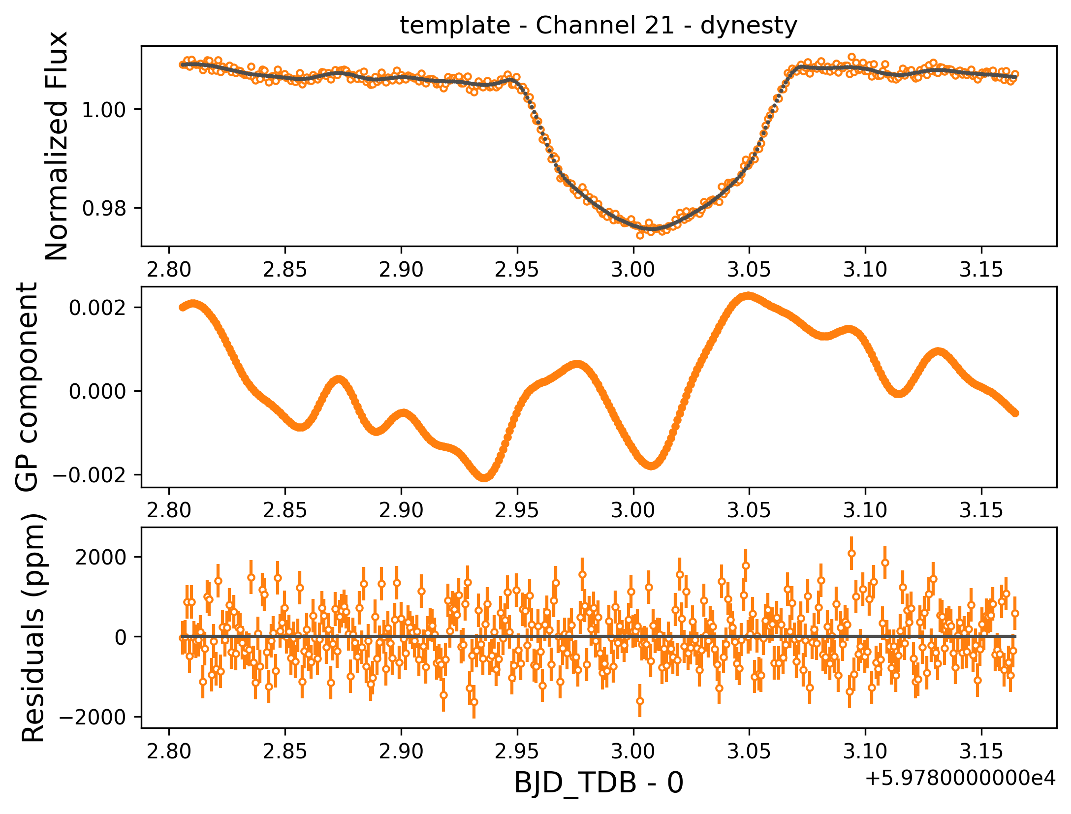
Fig 5102: Fitted Lightcurve, GP Model, and Residual Plot

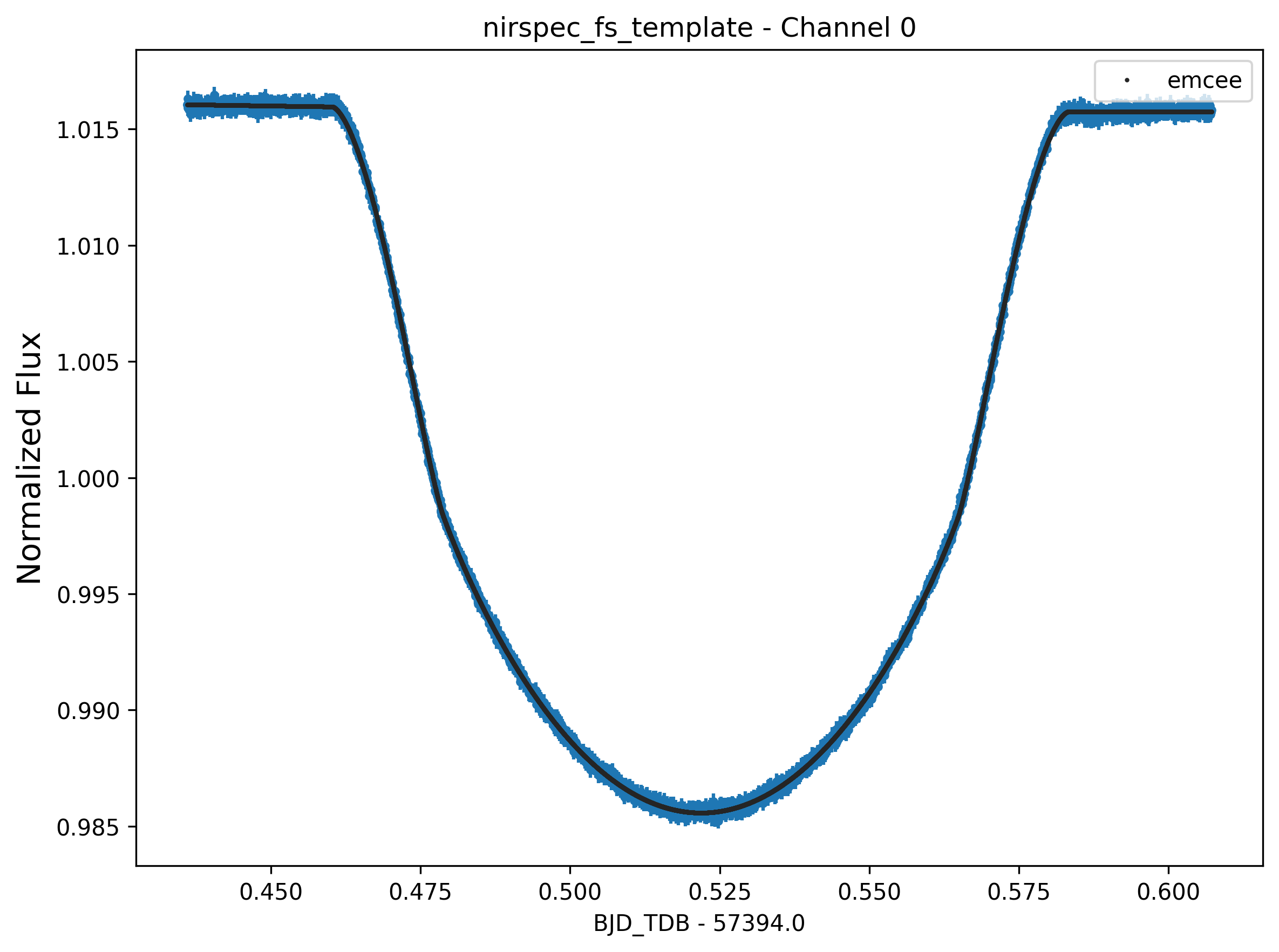
Fig 5103: Comparison of Different Fitters

Fig 5104: (Demo figure to come) Zoomed-in Figure Emphasizing Phase Variations Using Temporally Binned Data.

• If isplots_S5 = 3: Eureka! will plot an RMS deviation plot for each channel to help check for correlated noise, plot the normalized residual distribution, and plot the fitting chains for each channel. If fitting a sinusoid_pc model, another zoomed-in figure with binned data in front of the unbinned data will be made to emphasize the phase variations.

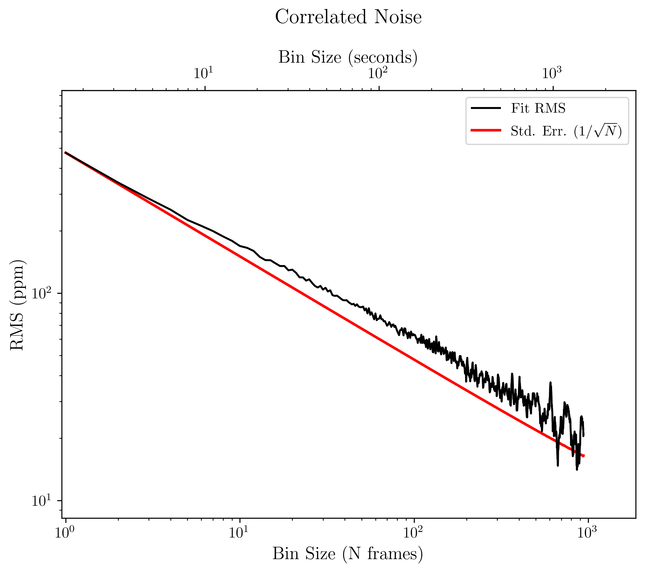
Fig 5301: RMS Deviation Plot

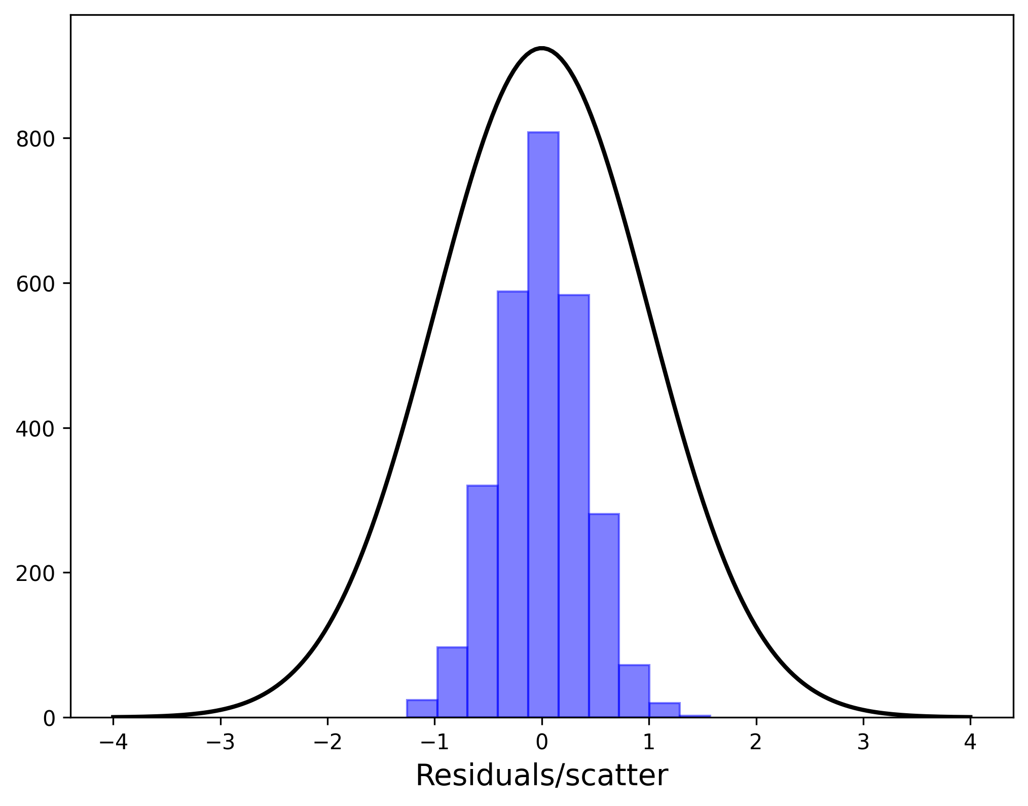
Fig 5302: Residual Distribution

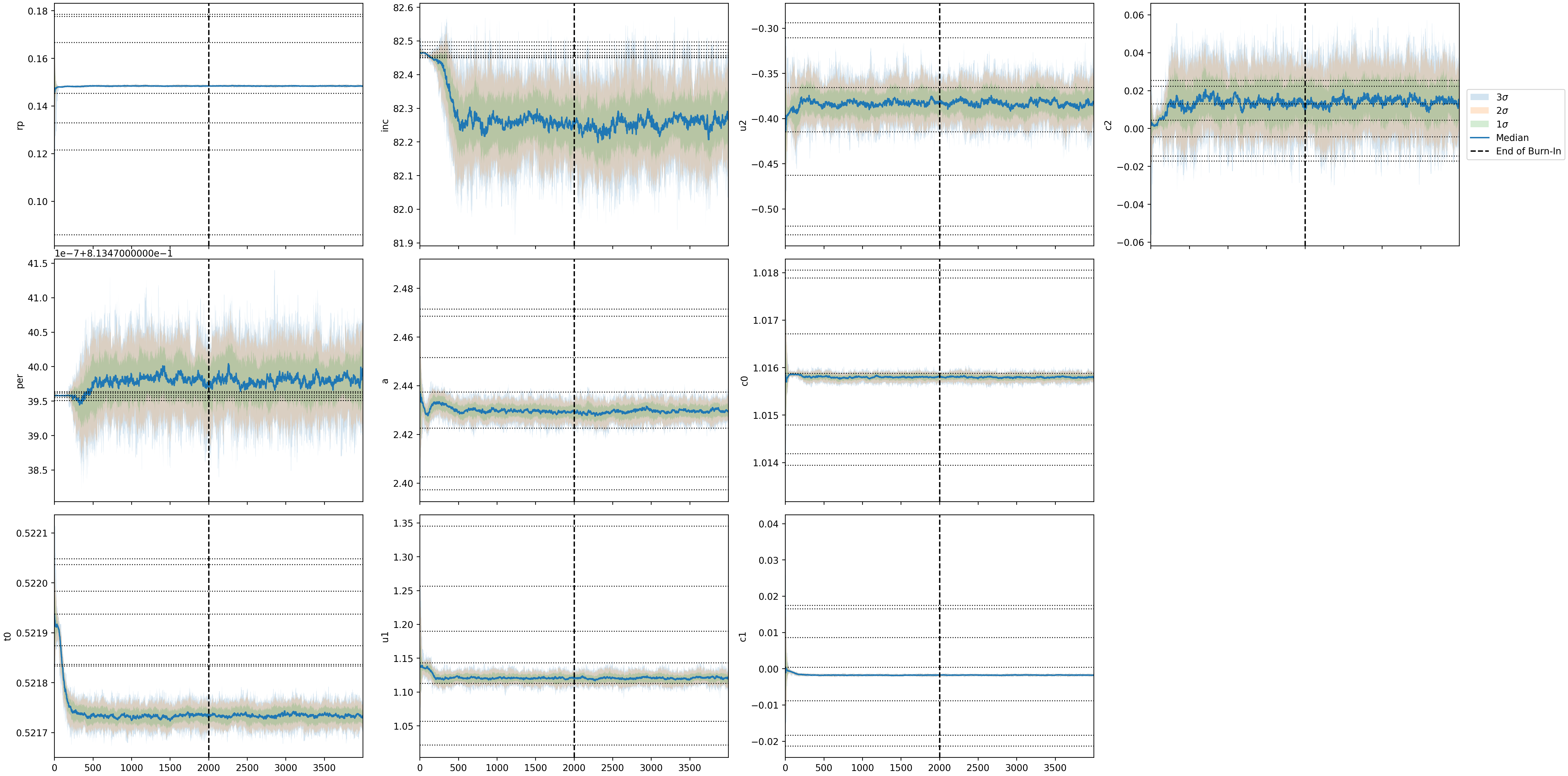
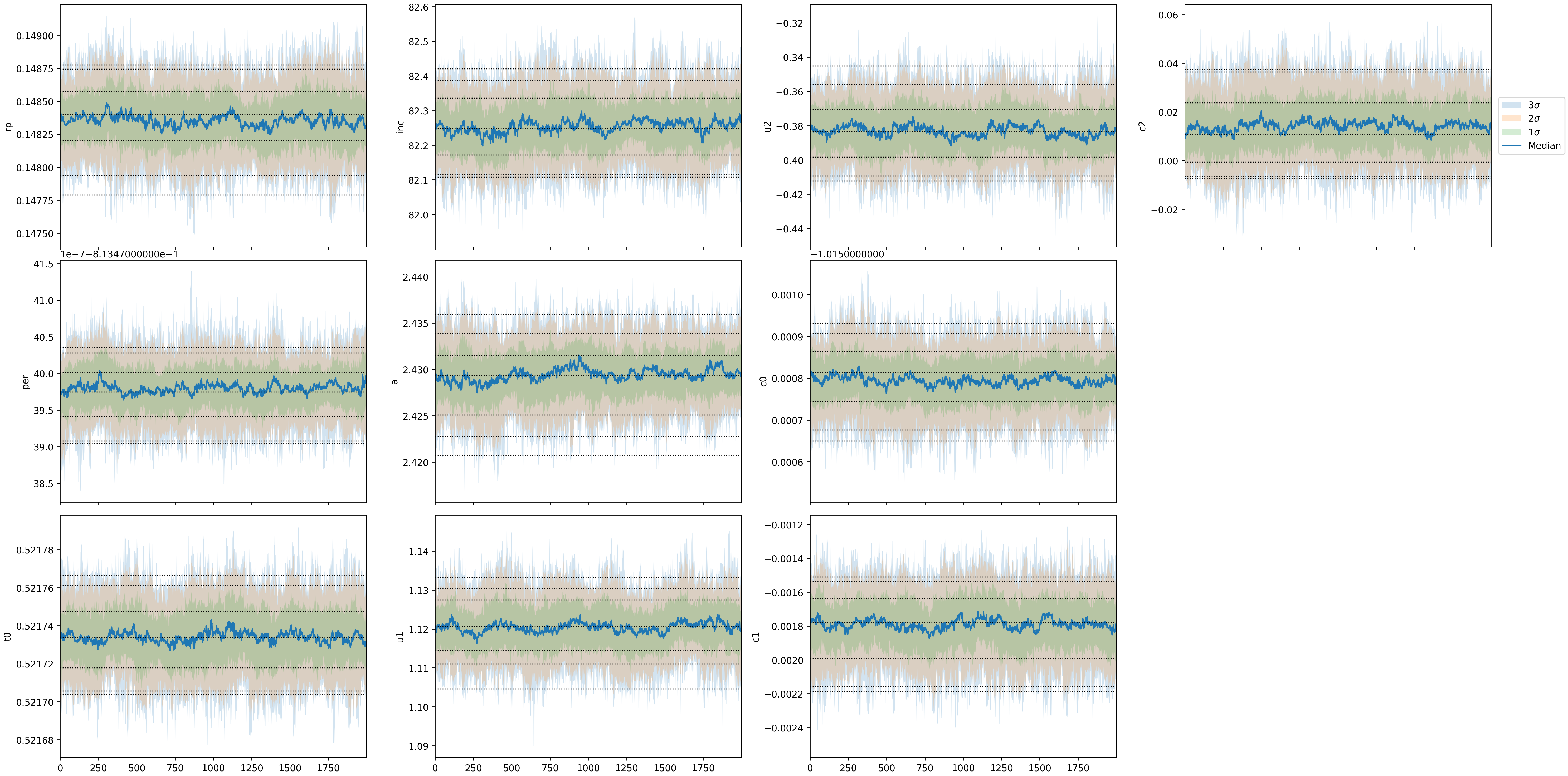
Figs 5303: Fitting Chains. Only made for emcee runs. Two version of the plot will be saved, one including the burn in steps and one without the burn in steps.

Fig 5304: (Demo figure to come) Zoomed-in Figure Emphasizing Phase Variations Using Temporally Binned Data Over Unbinned Data.

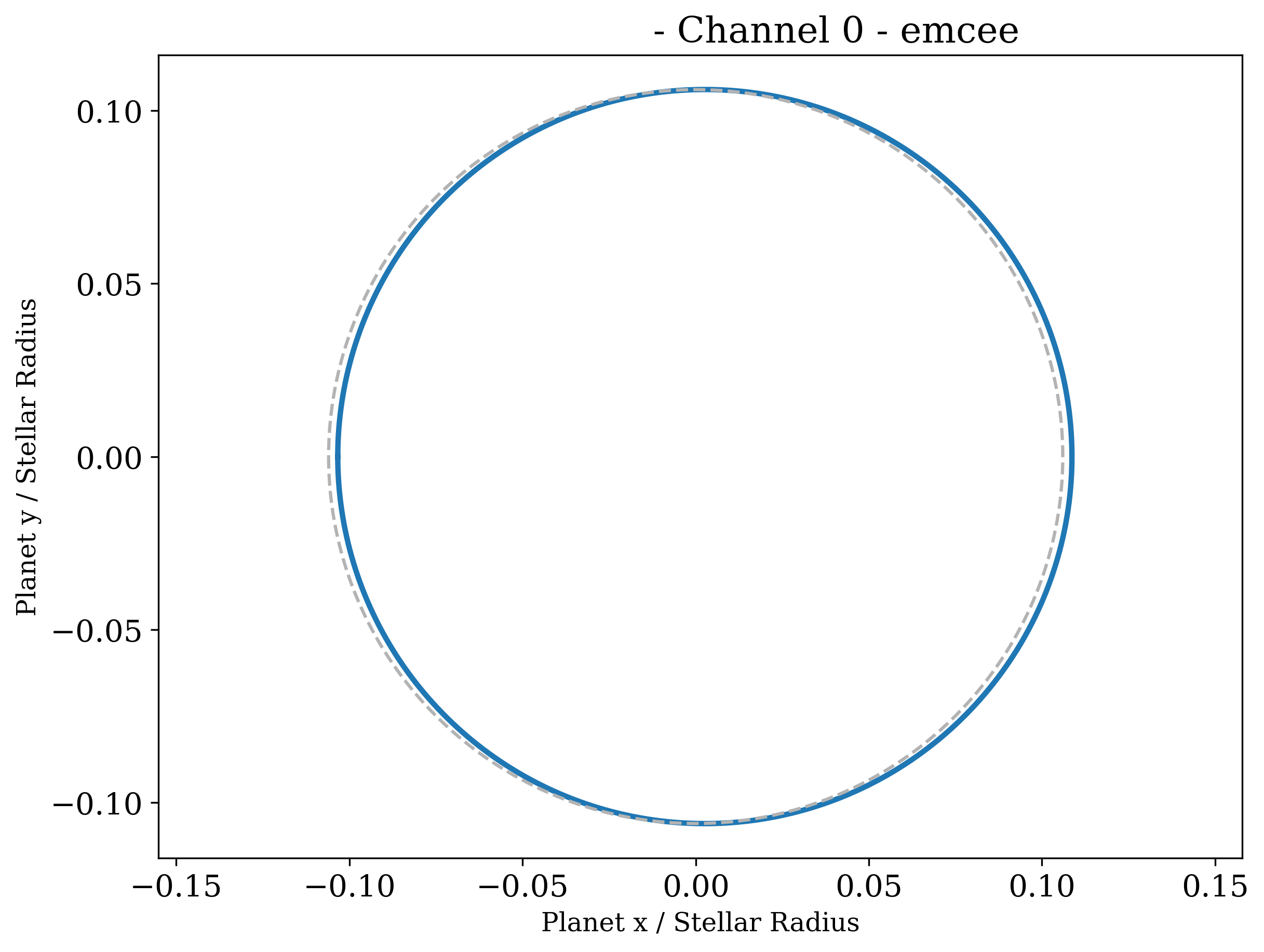
Fig 5309: Harmonica transmission string. The blue solid line depicts the measured shape of the planet. Any deviation from the reference circle (gray dashed line) points to a non-spherical planet. The morning limb is on the right; the evening limb is on the left.

• If isplots_S5 = 5, and if emcee or dynesty were used as the fitter: Eureka! will plot a corner plot for each channel.

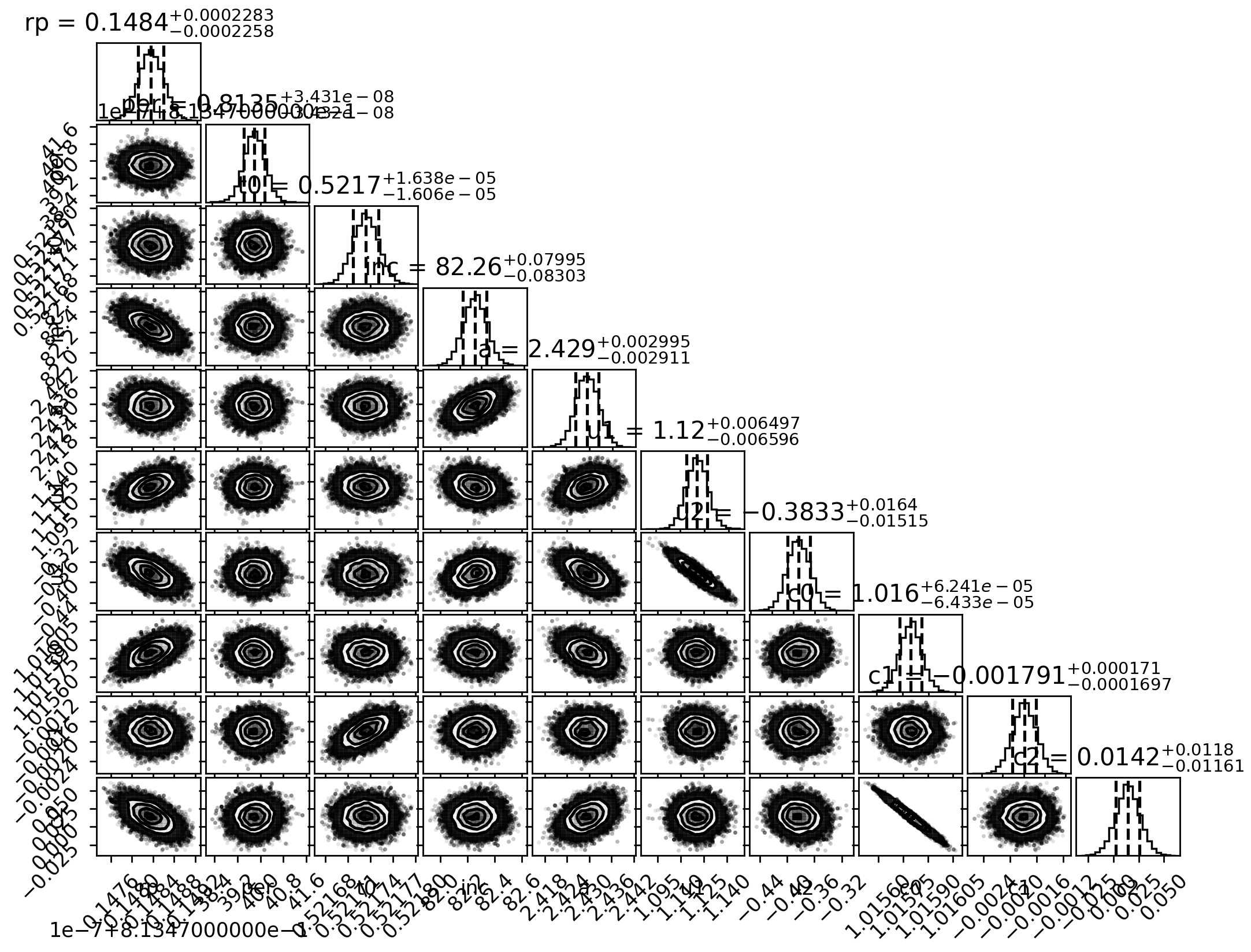
Fig 5501: Corner Plot

Stage 6 Outputs

In Stage 6:

• If isplots_S6 = 1: Eureka! will plot the transmission or emission spectrum, depending on the setting of y_unit. If a model is provided, it will be plotted on the same figure along with points binned from that model to the resolution of the data.

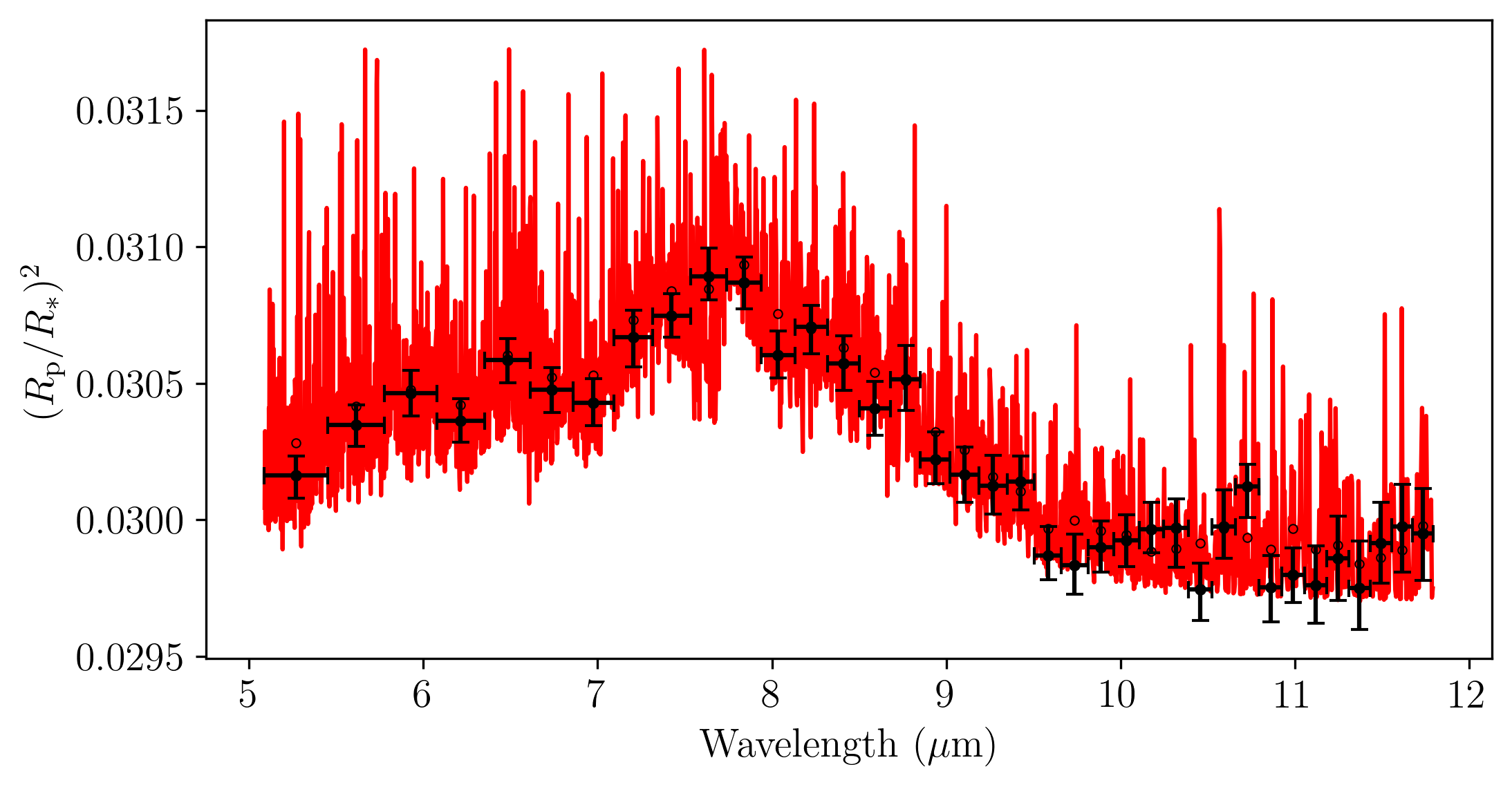
Fig 6101: Transmission Spectrum.

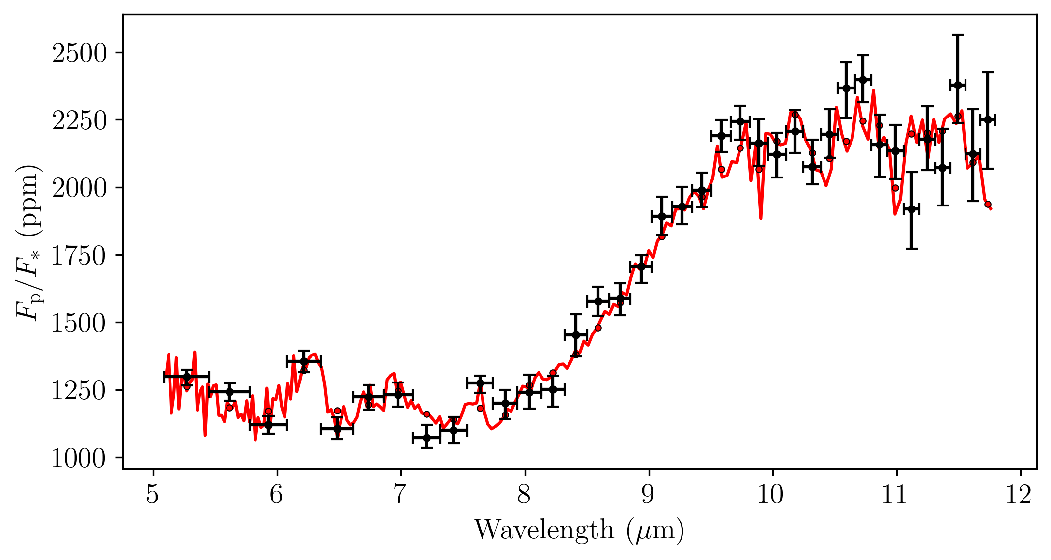
Fig 6101: Emission Spectrum.

• If isplots_S6 = 3: Eureka! will make another transmission plot (if y_unit is transmission type) with a second y-axis which is in units of atmospheric scale height.

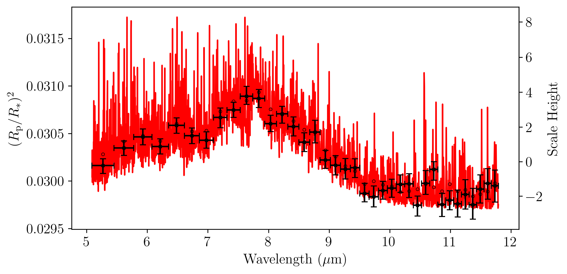
Fig 6301: Transmission Spectrum with Double y-axis.