Eureka! Control File (.ecf)
To run the different Stages of Eureka!, the pipeline requires control files (.ecf) where Stage-specific parameters are defined (e.g. aperture size, path of the data, etc.).
In the following, we look at the contents of the ecf for Stages 1, 2, 3, 4, 5, and 6.
Stage 1
# Eureka! Control File for Stage 1: Detector Processing

# Stage 1 Documentation: https://eurekadocs.readthedocs.io/en/latest/ecf.html#stage-1

suffix              uncal

# Control ramp fitting method
ramp_fit_algorithm  'default'   #Options are 'default', 'mean', or 'differenced'
ramp_fit_max_cores  'none'  #Options are 'none', quarter', 'half','all'

# Pipeline stages
skip_group_scale    False
skip_dq_init        False
skip_saturation     False
skip_ipc            True    #Skipped by default for all instruments
skip_superbias      False
skip_refpix         False
skip_linearity      False
skip_persistence    True    #Skipped by default for Near-IR TSO
skip_dark_current   False
skip_jump           False
skip_ramp_fitting   False
skip_gain_scale     False

#Pipeline stages parameters
jump_rejection_threshold  4.0 #float, default is 4.0, CR sigma rejection threshold

# Project directory
topdir              /home/User

# Directories relative to topdir
inputdir            /Data/JWST-Sim/NIRSpec/Uncalibrated
outputdir           /Data/JWST-Sim/NIRSpec/Stage1

# Diagnostics
testing_S1          False

#####

# "Default" ramp fitting settings
default_ramp_fit_weighting          default             #Options are "default", "fixed", "interpolated", "flat", or "custom"
default_ramp_fit_fixed_exponent     10                  #Only used for "fixed" weighting
default_ramp_fit_custom_snr_bounds  [5,10,20,50,100]    # Only used for "custom" weighting, array no spaces
default_ramp_fit_custom_exponents   [0.4,1,3,6,10]      # Only used for "custom" weighting, array no spaces
suffix
Data file suffix (e.g. uncal).
ramp_fit_algorithm
Algorithm to use to fit a ramp to the frame-level images of uncalibrated files. Only default (i.e. the JWST pipeline) and mean can be used currently.
ramp_fit_max_cores
Fraction of processor cores to use to compute the ramp fits, options are none, quarter, half, all.
skip_*
If True, skip the named step.
Note
Note that some instruments and observing modes might skip a step either way! See here for the list of steps run for each instrument/mode by the STScI’s JWST pipeline.
topdir + inputdir
The path to the directory containing the Stage 0 JWST data (uncal.fits).
topdir + outputdir
The path to the directory in which to output the Stage 1 JWST data and plots.
testing_S1
If True, only a single file will be used, outputs won’t be saved, and plots won’t be made. Useful for making sure most of the code can run.
default_ramp_fit_weighting
Define the method by which individual frame pixels will be weighted during the default ramp fitting process. The is specifically for the case where ramp_fit_algorithm is default. Options are default, fixed, interpolated, flat, or custom.
default: Slope estimation using a least-squares algorithm with an “optimal” weighting, see here.
In short this weights each pixel, \(i\), within a slope following \(w_i = (i - i_{midpoint})^P\), where the exponent \(P\) is selected depending on the estimated signal-to-noise ratio of each pixel (see link above).
fixed: As with default, except the weighting exponent \(P\) is fixed to a precise value through the default_ramp_fit_fixed_exponent entry
interpolated: As with default, except the SNR to \(P\) lookup table is converted to a smooth interpolation.
flat: As with default, except the weighting equation is no longer used, and all pixels are weighted equally.
custom: As with default, except a custom SNR to \(P\) lookup table can be defined through the default_ramp_fit_custom_snr_bounds and default_ramp_fit_custom_exponents (see example .ecf file).
Stage 2
A full description of the Stage 2 Outputs is available here: Stage 2 Output
# Eureka! Control File for Stage 2: Data Reduction

# Stage 2 Documentation: https://eurekadocs.readthedocs.io/en/latest/ecf.html#stage-2

suffix                  rateints    # Data file suffix

# Controls the cross-dispersion extraction
slit_y_low              -1      # Use None to rely on the default parameters
slit_y_high             50      # Use None to rely on the default parameters

# Modify the existing file to change the dispersion extraction - FIX: DOES NOT WORK CURRENTLY
waverange_start         6e-08   # Use None to rely on the default parameters
waverange_end           6e-06   # Use None to rely on the default parameters

# Note: different instruments and modes will use different steps by default
skip_bkg_subtract       True    # Not run for TSO observations
skip_imprint_subtract   True    # Not run for NIRSpec Fixed Slit
skip_msa_flagging       True    # Not run for NIRSpec Fixed Slit
skip_extract_2d         False
skip_srctype            False
skip_master_background  True    # Not run for NIRSpec Fixed Slit
skip_wavecorr           False
skip_flat_field         True    # ***NOTE*** At the time the NIRSpec ERS Hackathon simulated data was created, this step did not work correctly and is by default turned off.
skip_straylight         True    # Not run for NIRSpec Fixed Slit
skip_fringe             True    # Not run for NIRSpec Fixed Slit
skip_pathloss           True    # Not run for TSO observations
skip_barshadow          True    # Not run for NIRSpec Fixed Slit
skip_photom             True    # Recommended to skip to get better uncertainties out of Stage 3.
skip_resample           True    # Not run for TSO observations
skip_cube_build         True    # Not run for NIRSpec Fixed Slit
skip_extract_1d         False

# Diagnostics
testing_S2              False
hide_plots              False   # If True, plots will automatically be closed rather than popping up

# Project directory
topdir                  /home/User/

# Directories relative to topdir
inputdir                /Data/JWST-Sim/NIRSpec/Stage1
outputdir               /Data/JWST-Sim/NIRSpec/Stage2
suffix
Data file suffix (e.g. rateints).
Note
Note that other Instruments might used different suffixes!
slit_y_low & slit_y_high
Controls the cross-dispersion extraction. Use None to rely on the default parameters.
waverange_start & waverange_end
Modify the existing file to change the dispersion extraction (DOES NOT WORK). Use None to rely on the default parameters.
skip_*
If True, skip the named step.
Note
Note that some instruments and observing modes might skip a step either way! See here for the list of steps run for each instrument/mode by the STScI’s JWST pipeline.
testing_S2
If True, outputs won’t be saved and plots won’t be made. Useful for making sure most of the code can run.
hide_plots
If True, plots will automatically be closed rather than popping up on the screen.
topdir + inputdir
The path to the directory containing the Stage 1 JWST data.
topdir + outputdir
The path to the directory in which to output the Stage 2 JWST data and plots.
Stage 3
# Eureka! Control File for Stage 3: Data Reduction

# Stage 3 Documentation: https://eurekadocs.readthedocs.io/en/latest/ecf.html#stage-3

ncpu            1           # Number of CPUs
nfiles          1           # The number of data files to analyze simultaneously
max_memory      0.5         # The maximum fraction of memory you want utilized by read-in frames (this will reduce nfiles if need be)
suffix          calints     # Data file suffix

# Subarray region of interest
ywindow         [2,28]      # Vertical axis as seen in DS9
xwindow         [60,410]    # Horizontal axis as seen in DS9
src_pos_type    gaussian    # Determine source position when not given in header (Options: header, gaussian, weighted, max, or hst)

# Background parameters
bg_hw           7           # Half-width of exclusion region for BG subtraction (relative to source position)
bg_thresh       [10,10]     # Double-iteration X-sigma threshold for outlier rejection along time axis
bg_deg          1           # Polynomial order for column-by-column background subtraction, -1 for median of entire frame
p3thresh        10          # X-sigma threshold for outlier rejection during background subtraction
save_bgsub      False       # Whether or not to save background subtracted FITS files

# Spectral extraction parameters
record_ypos     False       # Option to record the y position and width for each integration (only records if src_pos_type is gaussian)
spec_hw         6           # Half-width of aperture region for spectral extraction (relative to source position)
fittype         smooth      # Method for constructing spatial profile (Options: smooth, meddata, poly, gauss, wavelet, or wavelet2D)
window_len      11          # Smoothing window length, when fittype = smooth
prof_deg        3           # Polynomial degree, when fittype = poly
p5thresh        10          # X-sigma threshold for outlier rejection while constructing spatial profile
p7thresh        60          # X-sigma threshold for outlier rejection during optimal spectral extraction

# G395H curvature treatment
curvature       correct     # How to manage the curved trace on the detector (Options: None, correct)

# Diagnostics
isplots_S3      3           # Generate few (1), some (3), or many (5) figures (Options: 1 - 5)
vmin            0.97        # Sets the vmin of the color bar for Figure 3101.
vmax            1.03        # Sets the vmax of the color bar for Figure 3101.
time_axis       'y'         # Determines whether the time axis in Figure 3101 is along the y-axis ('y') or the x-axis ('x')
testing_S3      False       # Boolean, set True to only use last file and generate select figures
hide_plots      False       # If True, plots will automatically be closed rather than popping up
save_output     True        # Save outputs for use in S4
verbose         True        # If True, more details will be printed about steps

# Project directory
topdir          /home/User/

# Directories relative to topdir
inputdir        /Data/JWST-Sim/NIRSpec/Stage2/   # The folder containing the outputs from Eureka!'s S2 or JWST's S2 pipeline (will be overwritten if calling S2 and S3 sequentially)
outputdir       /Data/JWST-Sim/NIRSpec/Stage3/
ncpu
Sets the number of cores being used when Eureka! is executed.
Currently, the only parallelized part of the code is the background subtraction for every individual integration and is being initialized in s3_reduce.py with:
util.BGsubtraction
nfiles
Sets the maximum number of data files to analyze batched together.
max_memory
Sets the maximum memory fraction (0–1) that should be used by the loaded in data files. This will reduce nfiles if needed. Note that more RAM than this may be used during operations like sigma clipping, so you’re best off setting max_memory <= 0.5.
suffix
If your data directory (topdir + inputdir, see below) contains files with different data formats, you want to consider setting this variable.
E.g.: Simulated NIRCam Data:
Stage 2 - For NIRCam, Stage 2 consists of the flat field correction, WCS/wavelength solution, and photometric calibration (counts/sec -> MJy). Note that this is specifically for NIRCam: the steps in Stage 2 change a bit depending on the instrument. The Stage 2 outputs are roughly equivalent to a “flt” file from HST.
Stage 2 Outputs/*calints.fits- Fully calibrated images (MJy) for each individual integration. This is the one you want if you’re starting with Stage 2 and want to do your own spectral extraction.Stage 2 Outputs/*x1dints.fits- A FITS binary table containing 1D extracted spectra for each integration in the “calint” files.
As we want to do our own spectral extraction, we set this variable to calints.
Note
Note that other Instruments might used different suffixes!
hst_cal
Only used for HST analyses. The fully qualified path to the folder containing HST calibration files.
horizonsfile
Only used for HST analyses. The path with respect to hst_cal to the horizons file you’ve downloaded from https://ssd.jpl.nasa.gov/horizons/app.html#/. To get a new horizons file on that website, 1. Select “Vector Table”, 2. Select “HST”, 3. Select “@ssb” (Solar System Barycenter), 4. Select a date range that spans the days relevant to your observations. Then click Generate Ephemeris and click Download Results.
leapdir
Only used for HST analyses. The folder with respect to hst_cal where leapsecond calibration files will be saved.
flatfile
Only used for HST analyses. The path with respect to hst_cal to the flatfield file to use. A WFC3/G102 flat can be downloaded here and a WFC3/G141 flat can be downloaded here; be sure to unzip the files after downloading them.
ywindow & xwindow
Can be set if one wants to remove edge effects (e.g.: many nans at the edges).
Below an example with the following setting:
ywindow     [5,64]
xwindow     [100,1700]
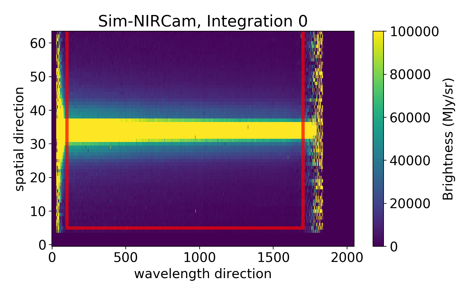
Everything outside of the box will be discarded and not used in the analysis.
src_pos_type
Determine the source position on the detector. Options: header, gaussian, weighted, max, or hst. The value ‘header’ uses the value of SRCYPOS in the FITS header.
centroidtrim
Only used for HST analyses. The box width to cut around the centroid guess to perform centroiding on the direct images. This should be an integer.
centroidguess
Only used for HST analyses. A guess for the location of the star in the direct images in the format [x, y].
flatoffset
Only used for HST analyses. The positional offset to use for flatfielding. This should be formatted as a 2 element list with x and y offsets.
flatsigma
Only used for HST analyses. Used to sigma clip bad values from the flatfield image.
diffthresh
Only used for HST analyses. Sigma theshold for bad pixel identification in the differential non-destructive reads (NDRs).
record_ypos
Option to record the cross-dispersion trace position and width (if Gaussian fit) for each integration.
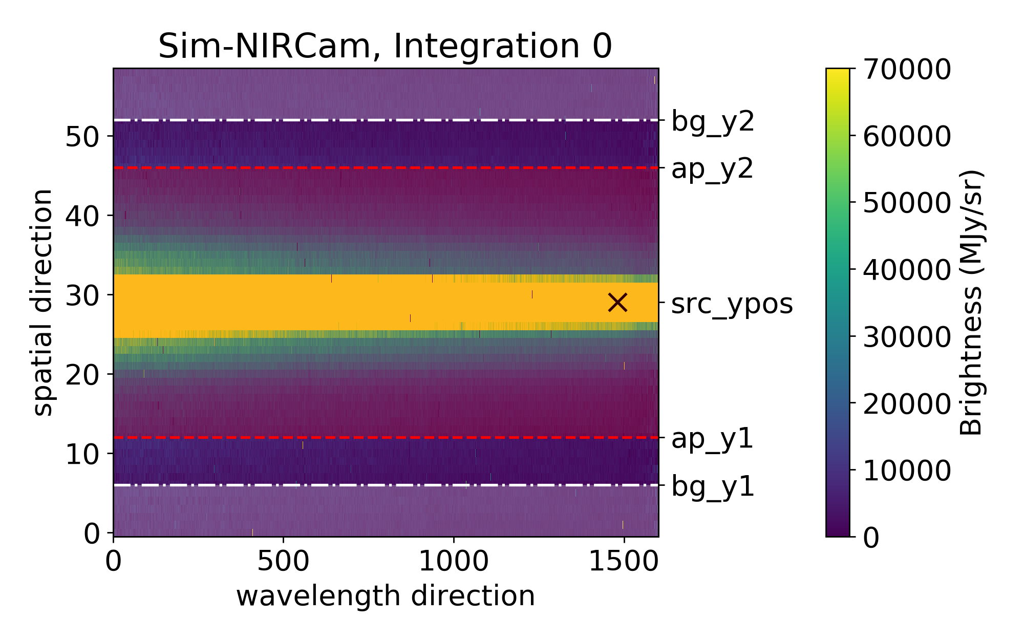
bg_hw & spec_hw
bg_hw and spec_hw set the background and spectrum aperture relative to the source position.
Let’s looks at an example with the following settings:
bg_hw    = 23
spec_hw  = 18
Looking at the fits file science header, we can determine the source position:
src_xpos = hdulist['SCI',1].header['SRCXPOS']-xwindow[0]
src_ypos = hdulist['SCI',1].header['SRCYPOS']-ywindow[0]
Let’s assume in our example that src_ypos = 29.
(xwindow[0] and ywindow[0] corrects for the trimming of the data frame, as the edges were removed with the xwindow and ywindow parameters)
The plot below shows you which parts will be used for the background calculation (shaded in white; between the lower edge and src_ypos - bg_hw, and src_ypos + bg_hw and the upper edge) and which for the spectrum flux calculation (shaded in red; between src_ypos - spec_hw and src_ypos + spec_hw).
bg_thresh
Double-iteration X-sigma threshold for outlier rejection along time axis.
The flux of every background pixel will be considered over time for the current data segment.
e.g: bg_thresh = [5,5]: Two iterations of 5-sigma clipping will be performed in time for every background pixel. Outliers will be masked and not considered in the background flux calculation.
bg_deg
Sets the degree of the column-by-column background subtraction. If bg_deg is negative, use the median background of entire frame. Set to None for no background subtraction. Also, best to emphasize that we’re performing column-by-column BG subtraction
The function is defined in S3_data_reduction.optspex.fitbg
Possible values:
bg_deg = None: No backgound subtraction will be performed.bg_deg < 0: The median flux value in the background area will be calculated and subtracted from the entire 2D Frame for this paticular integration.bg_deg => 0: A polynomial of degree bg_deg will be fitted to every background column (background at a specific wavelength). If the background data has an outlier (or several) which is (are) greater than 5 * (Mean Absolute Deviation), this value will be not considered as part of the background. Step-by-step:
Take background pixels of first column
Fit a polynomial of degree
bg_degto the background pixels.Calculate the residuals (flux(bg_pixels) - polynomial_bg_deg(bg_pixels))
Calculate the MAD (Mean Absolute Deviation) of the greatest background outlier.
If MAD of the greatest background outlier is greater than 5, remove this background pixel from the background value calculation. Repeat from Step 2. and repeat as long as there is no 5*MAD outlier in the background column.
Calculate the flux of the polynomial of degree
bg_deg(calculated in Step 2) at the spectrum and subtract it.
p3thresh
Only important if bg_deg => 0 (see above). # sigma threshold for outlier rejection during background subtraction which corresponds to step 3 of optimal spectral extraction, as defined by Horne (1986).
p5thresh
Used during Optimal Extraction. # sigma threshold for outlier rejection during step 5 of optimal spectral extraction, as defined by Horne (1986). Default is 10. For more information, see the source code of optspex.optimize.
p7thresh
Used during Optimal Extraction. # sigma threshold for outlier rejection during step 7 of optimal spectral extraction, as defined by Horne (1986). Default is 10. For more information, see the source code of optspex.optimize.
fittype
Used during Optimal Extraction. fittype defines how to construct the normalized spatial profile for optimal spectral extraction. Options are: ‘smooth’, ‘meddata’, ‘wavelet’, ‘wavelet2D’, ‘gauss’, or ‘poly’. Using the median frame (meddata) should work well with JWST. Otherwise, using a smoothing function (smooth) is the most robust and versatile option. Default is meddata. For more information, see the source code of optspex.optimize.
window_len
Used during Optimal Extraction. window_len is only used when fittype = ‘smooth’. It sets the length scale over which the data are smoothed. Default is 31. For more information, see the source code of optspex.optimize.
prof_deg
Used during Optimal Extraction. prof_deg is only used when fittype = ‘poly’. It sets the polynomial degree when constructing the spatial profile. Default is 3. For more information, see the source code of optspex.optimize.
iref
Only used for HST analyses. The file indices to use as reference frames for 2D drift correction. This should be a 1-2 element list with the reference indices for each scan direction.
curvature
Used only for G395H observations which display curvature in the trace. Current options: ‘None’, ‘correct’. Using ‘None’ will turn off any curvature correction and is included for users with custom routines that will handle the curvature of the trace. Using ‘correct’ will bring the center of mass of each column to the center of the detector and perform the extraction on this straightened trace. This option should be used with fittype = ‘meddata’.
isplots_S3
Sets how many plots should be saved when running Stage 3. A full description of these outputs is available here: Stage 3 Output
vmin
Optional. Sets the vmin of the color bar for Figure 3101. Defaults to 0.97.
vmax
Optional. Sets the vmax of the color bar for Figure 3101. Defaults to 1.03.
time_axis
Optional. Determines whether the time axis in Figure 3101 is along the y-axis (‘y’) or the x-axis (‘x’). Defaults to ‘y’.
testing_S3
If set to True only the last segment (which is usually the smallest) in the inputdir will be run. Also, only five integrations from the last segment will be reduced.
save_output
If set to True output will be saved as files for use in S4. Setting this to False is useful for quick testing
hide_plots
If True, plots will automatically be closed rather than popping up on the screen.
verbose
If True, more details will be printed about steps.
topdir + inputdir
The path to the directory containing the Stage 2 JWST data. For HST observations, the sci_dir and cal_dir folders will only be checked if this folder does not contain FITS files.
topdir + inputdir + sci_dir
Optional, only used for HST analyses. The path to the folder containing the science spectra. Defaults to ‘sci’.
topdir + inputdir + cal_dir
Optional, only used for HST analyses. The path to the folder containing the wavelength calibration imaging mode observations. Defaults to ‘cal’.
topdir + outputdir
The path to the directory in which to output the Stage 3 JWST data and plots.
topdir + time_file
Optional. The path to a file that contains the time array you want to use instead of the one contained in the FITS file.
Stage 4
# Eureka! Control File for Stage 4: Generate Lightcurves

# Stage 4 Documentation: https://eurekadocs.readthedocs.io/en/latest/ecf.html#stage-4

# Number of spectroscopic channels spread evenly over given wavelength range
nspecchan       2           # Number of spectroscopic channels
compute_white   True        # Also compute the white-light lightcurve
wave_min        1.5         # Minimum wavelength. Set to None to use the shortest extracted wavelength from Stage 3.
wave_max        4.5         # Maximum wavelength. Set to None to use the longest extracted wavelength from Stage 3.
allapers        False       # Run S4 on all of the apertures considered in S3? Otherwise will use newest output in the inputdir

# Parameters for drift correction of 1D spectra
recordDrift     False    # Set True to record drift/jitter in 1D spectra (always recorded if correctDrift is True)
correctDrift    False   # Set True to correct drift/jitter in 1D spectra (not recommended for simulated data)
drift_preclip   0       # Ignore first drift_preclip points of spectrum
drift_postclip  100     # Ignore last drift_postclip points of spectrum, None = no clipping
drift_range     11      # Trim spectra by +/-X pixels to compute valid region of cross correlation
drift_hw        5       # Half-width in pixels used when fitting Gaussian, must be smaller than drift_range
drift_iref      -1      # Index of reference spectrum used for cross correlation, -1 = last spectrum
sub_mean        True    # Set True to subtract spectrum mean during cross correlation
sub_continuum   True    # Set True to subtract the continuum from the spectra using a highpass filter
highpassWidth   10      # The integer width of the highpass filter when subtracting the continuum

# Parameters for sigma clipping
sigma_clip      False   # Whether or not sigma clipping should be performed on the 1D time series
sigma           10      # The number of sigmas a point must be from the rolling median to be considered an outlier
box_width       10      # The width of the box-car filter (used to calculated the rolling median) in units of number of data points
maxiters        5       # The number of iterations of sigma clipping that should be performed.
boundary        'fill'  # Use 'fill' to extend the boundary values by the median of all data points (recommended), 'wrap' to use a periodic boundary, or 'extend' to use the first/last data points
fill_value      mask    # Either the string 'mask' to mask the outlier values (recommended), 'boxcar' to replace data with the mean from the box-car filter, or a constant float-type fill value.

# Limb-darkening parameters needed to compute exotic-ld
compute_ld      True
inst_filter     Prism #filter of JWST/HST instrument, supported list see https://exotic-ld.readthedocs.io/en/latest/views/supported_instruments.html
metallicity     0.1 #metallicity of the star
teff            6000 #effective temperature of the star in K
logg            4.0 #surface gravity in log g
exotic_ld_direc /home/User/exotic-ld_data/ #directory for ancillary files for exotic-ld
exotic_ld_grid  3D #1D or 3D model grid

# Diagnostics
isplots_S4      3       # Generate few (1), some (3), or many (5) figures (Options: 1 - 5)
vmin            0.97    # Sets the vmin of the color bar for Figure 4101.
vmax            1.03    # Sets the vmax of the color bar for Figure 4101.
time_axis       'y'     # Determines whether the time axis in Figure 4101 is along the y-axis ('y') or the x-axis ('x')
hide_plots      False   # If True, plots will automatically be closed rather than popping up
verbose         True    # If True, more details will be printed about steps

# Project directory
topdir          /home/User

# Directories relative to topdir
inputdir        /Data/JWST-Sim/NIRSpec/Stage3    # The folder containing the outputs from Eureka!'s S3 or JWST's S3 pipeline (will be overwritten if calling S3 and S4 sequentially)
outputdir       /Data/JWST-Sim/NIRSpec/Stage4
nspecchan
Number of spectroscopic channels spread evenly over given wavelength range
compute_white
If True, also compute the white-light lightcurve.
wave_min & wave_max
Start and End of the wavelength range being considered. Set to None to use the shortest/longest extracted wavelength from Stage 3.
allapers
If True, run S4 on all of the apertures considered in S3. Otherwise the code will use the only or newest S3 outputs found in the inputdir. To specify a particular S3 save file, ensure that “inputdir” points to the procedurally generated folder containing that save file (e.g. set inputdir to /Data/JWST-Sim/NIRCam/Stage3/S3_2021-11-08_nircam_wfss_ap10_bg10_run1/).
recordDrift
If True, compute drift/jitter in 1D spectra (always recorded if correctDrift is True)
correctDrift
If True, correct for drift/jitter in 1D spectra.
drift_preclip
Ignore first drift_preclip points of spectrum when correcting for drift/jitter in 1D spectra.
drift_postclip
Ignore the last drift_postclip points of spectrum when correcting for drift/jitter in 1D spectra. None = no clipping.
drift_range
Trim spectra by +/- drift_range pixels to compute valid region of cross correlation when correcting for drift/jitter in 1D spectra.
drift_hw
Half-width in pixels used when fitting Gaussian when correcting for drift/jitter in 1D spectra. Must be smaller than drift_range.
drift_iref
Index of reference spectrum used for cross correlation when correcting for drift/jitter in 1D spectra. -1 = last spectrum.
sub_mean
If True, subtract spectrum mean during cross correlation (can help with cross-correlation step).
sub_continuum
Set True to subtract the continuum from the spectra using a highpass filter
highpassWidth
The integer width of the highpass filter when subtracting the continuum
sigma_clip
Whether or not sigma clipping should be performed on the 1D time series
sigma
Only used if sigma_clip=True. The number of sigmas a point must be from the rolling median to be considered an outlier
box_width
Only used if sigma_clip=True. The width of the box-car filter (used to calculated the rolling median) in units of number of data points
maxiters
Only used if sigma_clip=True. The number of iterations of sigma clipping that should be performed.
boundary
Only used if sigma_clip=True. Use ‘fill’ to extend the boundary values by the median of all data points (recommended), ‘wrap’ to use a periodic boundary, or ‘extend’ to use the first/last data points
fill_value
Only used if sigma_clip=True. Either the string ‘mask’ to mask the outlier values (recommended), ‘boxcar’ to replace data with the mean from the box-car filter, or a constant float-type fill value.
sum_reads
Only used for HST analyses. Should differential non-destructive reads be summed together to reduce noise and data volume or not.
compute_ld
Whether or not to compute limb-darkening coefficients using exotic-ld.
inst_filter
Used by exotic-ld if compute_ld=True. The filter of JWST/HST instrument, supported list see https://exotic-ld.readthedocs.io/en/latest/views/supported_instruments.html (leave off the observatory and instrument so that JWST_NIRSpec_Prism becomes just Prism).
metallicity
Used by exotic-ld if compute_ld=True. The metallicity of the star.
teff
Used by exotic-ld if compute_ld=True. The effective temperature of the star in K.
logg
Used by exotic-ld if compute_ld=True. The surface gravity in log g.
exotic_ld_direc
Used by exotic-ld if compute_ld=True. The fully qualified path to the directory for ancillary files for exotic-ld.
exotic_ld_grid
Used by exotic-ld if compute_ld=True. 1D or 3D model grid.
isplots_S4
Sets how many plots should be saved when running Stage 4. A full description of these outputs is available here: Stage 4 Output
vmin
Optional. Sets the vmin of the color bar for Figure 4101. Defaults to 0.97.
vmax
Optional. Sets the vmax of the color bar for Figure 4101. Defaults to 1.03.
time_axis
Optional. Determines whether the time axis in Figure 4101 is along the y-axis (‘y’) or the x-axis (‘x’). Defaults to ‘y’.
hide_plots
If True, plots will automatically be closed rather than popping up on the screen.
verbose
If True, more details will be printed about steps.
topdir + inputdir
The path to the directory containing the Stage 3 JWST data.
topdir + outputdir
The path to the directory in which to output the Stage 4 JWST data and plots.
Stage 5
# Eureka! Control File for Stage 5: Lightcurve Fitting

# Stage 5 Documentation: https://eurekadocs.readthedocs.io/en/latest/ecf.html#stage-5

ncpu            1 # The number of CPU threads to use when running emcee or dynesty in parallel

allapers        False                   # Run S5 on all of the apertures considered in S4? Otherwise will use newest output in the inputdir
rescale_err     False                   # Rescale uncertainties to have reduced chi-squared of unity
fit_par         ./S5_fit_par_template.epf   # What fitting epf do you want to use?
verbose         True                    # If True, more details will be printed about steps
fit_method      [dynesty]               #options are: lsq, emcee, dynesty (can list multiple types separated by commas)
run_myfuncs     [batman_tr,polynomial]  #options are: batman_tr, batman_ecl, sinusoid_pc, expramp, GP, and polynomial (can list multiple types separated by commas)

# Limb darkening controls
use_generate_ld  exotic-ld #use the generated limb-darkening coefficients from Stage 4? Options: exotic-ld, None
#important: limb-darkening coefficients are not automatically fixed then, change to 'fixed' in .epf file whether they should be fixed or fitted! The limb-darkening laws available are linear, quadratic, 3-parameter and 4-parameter non-linear.
#(not yet implemented)
#fix_ld          True #use limb darkening file?
#ld_file         /path/to/limbdarkening/ld_outputfile.txt  #location of limb darkening file

# General fitter
old_fitparams   None # filename relative to topdir that points to a fitparams csv to resume where you left off (set to None to start from scratch)

#lsq
lsq_method      'Nelder-Mead' # The scipy.optimize.minimize optimization method to use
lsq_tol         1e-6    # The tolerance for the scipy.optimize.minimize optimization method
lsq_maxiter     None    # Maximum number of iterations to perform. Depending on the method each iteration may use several function evaluations. Set to None to use the default value

#mcmc
old_chain       None    # Output folder relative to topdir that contains an old emcee chain to resume where you left off (set to None to start from scratch)
lsq_first       True    # Initialize with an initial lsq call (can help shorten burn-in, but turn off if lsq fails). Only used if old_chain is None
run_nsteps      1000
run_nwalkers    200
run_nburn       500     # How many of run_nsteps should be discarded as burn-in steps

#dynesty
run_nlive       1024    # Must be > ndim * (ndim + 1) // 2
run_bound       'multi'
run_sample      'auto'
run_tol         0.1

#GP inputs
kernel_inputs   ['time'] #options: time
kernel_class    ['Matern32'] #options: ExpSquared, Matern32, Exp, RationalQuadratic for george, Matern32 for celerite (sums of kernels possible for george separated by commas)
GP_package      'celerite' #options: george, celerite

# Plotting controls
interp          False   # Should astrophysical model be interpolated (useful for uneven sampling like that from HST)

# Diagnostics
isplots_S5      5       # Generate few (1), some (3), or many (5) figures (Options: 1 - 5)
testing_S5      False   # Boolean, set True to only use the first spectral channel
testing_model   False   # Boolean, set True to only inject a model source of systematics
hide_plots      False   # If True, plots will automatically be closed rather than popping up

# Project directory
topdir          /home/User

# Directories relative to topdir
inputdir        /Data/JWST-Sim/NIRSpec/Stage4/   # The folder containing the outputs from Eureka!'s S4 pipeline (will be overwritten if calling S4 and S5 sequentially)
outputdir       /Data/JWST-Sim/NIRSpec/Stage5/
ncpu
Integer. Sets the number of CPUs to use for multiprocessing Stage 5 fitting.
allapers
Boolean to determine whether Stage 5 is run on all the apertures considered in Stage 4. If False, will just use the most recent output in the input directory.
rescale_err
Boolean to determine whether the uncertainties will be rescaled to have a reduced chi-squared of 1
fit_par
Path to Stage 5 priors and fit parameter file.
verbose
If True, more details will be printed about steps.
fit_method
Fitting routines to run for Stage 5 lightcurve fitting. Can be one or more of the following: [lsq, emcee, dynesty]
run_myfuncs
Determines the transit and systematics models used in the Stage 5 fitting. Can be one or more of the following: [batman_tr, batman_ecl, sinusoid_pc, expramp, polynomial]
use_generate_ld
If you want to use the generated limb-darkening coefficients from Stage 4, use exotic-ld. Otherwise, use None. Important: limb-darkening coefficients are not automatically fixed, change the limb darkening parameters to ‘fixed’ in the .epf file if they should be fixed instead of fitted! The limb-darkening laws available to exotic-ld are linear, quadratic, 3-parameter and 4-parameter non-linear.
Least-Squares Fitting Parameters
The following set the parameters for running the least-squares fitter.
lsq_method
Least-squares fitting method: one of any of the scipy.optimize.minimize least-squares methods.
lsq_tolerance
Float to determine the tolerance of the scipy.optimize.minimize method.
Emcee Fitting Parameters
The following set the parameters for running emcee.
old_chain
Output folder containing previous emcee chains to resume previous runs. To start from scratch, set to None.
lsq_first
Boolean to determine whether to run least-squares fitting before MCMC. This can shorten burn-in but should be turned off if least-squares fails. Only used if old_chain is None.
run_nsteps
Integer. The number of steps for emcee to run.
run_nwalkers
Integer. The number of walkers to use.
run_nburn
Integer. The number of burn-in steps to run.
Dynesty Fitting Parameters
The following set the parameters for running dynesty. These options are described in more detail in: https://dynesty.readthedocs.io/en/latest/api.html?highlight=unif#module-dynesty.dynesty
run_nlive
Integer. Number of live points for dynesty to use. Should be at least greater than (ndim * (ndim+1)) / 2, where ndim is the total number of fitted parameters. For shared fits, multiply the number of free parameters by the number of wavelength bins specified in Stage 4.
run_bound
The bounding method to use. Options are: [‘none’, ‘single’, ‘multi’, ‘balls’, ‘cubes’]
run_sample
The sampling method to use. Options are [‘auto’, ‘unif’, ‘rwalk’, ‘rstagger’, ‘slice’, ‘rslice’, ‘hslice’]
run_tol
Float. The tolerance for the dynesty run. Determines the stopping criterion. The run will stop when the estimated contribution of the remaining prior volume to the total evidence falls below this threshold.
interp
Boolean to determine whether the astrophysical model is interpolated when plotted. This is useful when there is uneven sampling in the observed data.
isplots_S5
Sets how many plots should be saved when running Stage 5. A full description of these outputs is available here: Stage 5 Output
hide_plots
If True, plots will automatically be closed rather than popping up on the screen.
topdir + inputdir
The path to the directory containing the Stage 4 JWST data.
topdir + outputdir
The path to the directory in which to output the Stage 5 JWST data and plots.
Stage 5 Fit Parameters
Warning
The Stage 5 fit parameter file has the file extension .epf, not .ecf. These have different formats, and are not interchangeable.
This file describes the transit/eclipse and systematics parameters and their prior distributions. Each line describes a new parameter, with the following basic format:
Name Value Free PriorPar1 PriorPar2 PriorType
Namedefines the specific parameter being fit for. Available options are:- Transit and Eclipse Parameters
rp- planet-to-star radius ratio, for the transit models.fp- planet/star flux ratio, for the eclipse models.
- Orbital Parameters
per- orbital period (in days)t0- transit time (in days)time_offset- (optional), the absolute time offset of your time-series data (in days)inc- orbital inclination (in degrees)a- a/R*, the ratio of the semimajor axis to the stellar radiusecc- orbital eccentricityw- argument of periapsis (degrees)
- Phase Curve Parameters - the phase curve model allows for the addition of up to four sinusoids into a single phase curve
AmpCos1- Amplitude of the first cosineAmpSin1- Amplitude of the first sineAmpCos2- Amplitude of the second cosineAmpSin2- Amplitude of the second sine
- Limb Darkening Parameters
limb_dark- The limb darkening model to be used. Options are:['uniform', 'linear', 'quadratic', 'kipping2013', 'square-root', 'logarithmic', 'exponential', '4-parameter']uniformlimb-darkening has no parameters,linearhas a single parameteru1,quadratic,kipping2013,square-root,logarithmic, andexponentialhave two parametersu1, u2,4-parameterhas four parametersu1, u2, u3, u4
Systematics Parameters - Depending on the model specified in the Stage 5 ECF, set either polynomial model coefficients
c0--c9for 0th to 3rd order polynomials. The polynomial coefficients are numbered as increasing powers (i.e.c0a constant,c1linear, etc.). The x-values of the polynomial are the time with respect to the mean of the time of the lightcurve time array. Polynomial fits should include at leastc0for usable results. The exponential ramp model is defined as follows:r0*np.exp(-r1*time_local + r2) + r3*np.exp(-r4*time_local + r5) + 1, wherer0--r2describe the first ramp, andr3--r5the second.time_localis the time relative to the first frame of the dataset. If you only want to fit a single ramp, you can omitr3--r5or set them to0.White Noise Parameters - options are
scatter_multfor a multiplier to the expected noise from Stage 3 (recommended), orscatter_ppmto directly fit the noise level in ppm.
Free determines whether the parameter is fixed, free, white_fixed, white_free, independent, or shared.
fixed parameters are fixed in the fitting routine and not fit for.
free parameters are fit for according to the specified prior distribution, independently for each wavelength channel.
white_fixed and white_free parameters are first fit using free on the white-light light curve to update the prior for the parameter, and then treated as fixed or free (respectively) for the spectral fits.
shared parameters are fit for according to the specified prior distribution, but are common to all wavelength channels.
independent variables set auxiliary functions needed for the fitting routines.
The PriorType can be U (Uniform), LU (Log Uniform), or N (Normal). If U/LU, then PriorPar1 and PriorPar2 are the lower and upper limits of the prior distribution. If N, then PriorPar1 is the mean and PriorPar2 is the stadard deviation of the Gaussian prior.
Here’s an example fit parameter file:
# Stage 5 Fit Parameters Documentation: https://eurekadocs.readthedocs.io/en/latest/ecf.html#stage-5-fit-parameters


# Name       Value         Free?          PriorPar1    PriorPar2    PriorType
# "Free?" can be free, fixed, white_free, white_fixed, shared, or independent
# PriorType can be U (Uniform), LU (Log Uniform), or N (Normal).
# If U/LU, PriorPar1 and PriorPar2 represent upper and lower limits of the parameter/log(the parameter).
# If N, PriorPar1 is the mean and PriorPar2 is the standard deviation of a Gaussian prior.
#-------------------------------------------------------------------------------------------------------
#
# ------------------
# ** Transit/eclipse parameters **
# ------------------
rp           0.148          'free'         0.15         0.1          N
#fp           0.008          'free'         0           0.5          U
# ----------------------
# ** Phase curve parameters **
# ----------------------
#AmpCos1      0.4           'free'         0            1            U
#AmpSin1      0.01          'free'         -1           1            U
#AmpCos2      0.01          'free'         -1           1            U
#AmpSin2      0.01          'free'         -1           1            U
# ------------------
# ** Orbital parameters **
# ------------------
per          4.055259       'free'         4.055259     1e-5         N
t0           57394.524      'free'         57394.524    0.05         N
time_offset  0              'independent'
inc          87.83          'free'         87.83        0.25         N
a            10.9           'free'         10.9         1            N  # An incorrect a/R* seems to have been used in the simulations
ecc          0.0            'fixed'        0            1            U
w            90.            'fixed'        0            180          U
# -------------------------
# ** Limb darkening parameters **
# Choose limb_dark from ['uniform', 'linear', 'quadratic', 'kipping2013', 'square-root', 'logarithmic', 'exponential','3-parameter', '4-parameter']
# When using generated limb-darkening coefficients from exotic-ld choose from ['linear', 'quadratic', '3-parameter', '4-parameter']
# -------------------------
limb_dark    'kipping2013'  'independent'
u1           0.59           'free'         0            1            U
u2           0.84           'free'         0            1            U
# --------------------
# ** Systematic variables **
# polynomial model variables (c0--c9 for 0th--3rd order polynomials in time); Fitting at least c0 is very strongly recommended!
# expramp model variables (r0--r2 for one exponential ramp, r3--r5 for a second exponential ramp)
# GP model parameters (A, WN, m1, m2) in log scale
# --------------------
c0           1.015          'free'         1            0.05         N
c1           0              'free'         0            0.01          N
#A            -5             'free'         -20.         -5.          U
#WN           -15            'free'         -20.         -10.         U
#m1           -5             'free'         -10.         0.           U
# -----------
# ** White noise **
# Use scatter_mult to fit a multiplier to the expected noise level from Stage 3 (recommended)
# Use scatter_ppm to fit the noise level in ppm
# Use WN parameter in GP model parameters to account for white noise in the GP model
# -----------
#scatter_mult 1.1            'free'         1            0.1          N
scatter_ppm  500            'free'         500          100          N
Stage 6
# Eureka! Control File for Stage 6: Spectra Plotting

# Stage 6 Documentation: https://eurekadocs.readthedocs.io/en/latest/ecf.html#stage-6

allapers        False # Run S6 on all of the apertures considered in S5? Otherwise will use newest output in the inputdir

# Plotting parameters
y_unit          (Rp/Rs)^2 # Options include Rp/Rs, (Rp/Rs)^2, Fp/Fs
y_scalar        100 # Can be used to convert to percent (100), ppm (1e6), etc.
x_unit          um # Options include any measurement of light included in astropy.units.spectral (e.g. um, nm, Hz, etc.)

# This section is relevant if isplots_S6>=3
# Scale height parameters (if you want a second copy of the plot with a second y-axis with units of scale height)
star_Rad        0.6506 # The radius of the star in units of solar radii
planet_Teq      1400 # The equilibrium temperature of the planet in units of Kelvin
planet_Mass     2 # The planet's mass in units of Jupiter masses (used to calculate surface gravity)
planet_Rad      None # The planet's radius in units of Jupiter radii (used to calculate surface gravity); Set to None to use the average fitted radius
planet_mu       2.3 # The mean molecular mass of the atmosphere (in atomic mass units)
planet_R0       None # The reference radius (in Jupiter radii) for the scale height measurement; Set to None to use the mean fitted radius

# Diagnostics
isplots_S6      5 # Generate few (1), some (3), or many (5) figures (Options: 1 - 5)
hide_plots      False # If True, plots will automatically be closed rather than popping up

# Project directory
topdir          /home/User/

# Model to plot underneath the fitted data points
model_spectrum  None # Path to the model spectrum relative to topdir. Set to None if no model should be plotted.
model_x_unit    um # Options include any measurement of light included in astropy.units.spectral (e.g. um, nm, Hz, etc.)
model_y_unit    Rp/Rs # Options include Rp/Rs, (Rp/Rs)^2, Fp/Fs
model_y_scalar  1 # Indicate whether model y-values have already been scaled (e.g. write 1e6 if model_spectrum is in ppm)
model_zorder    0 # The zorder of the model on the plot (0 for beneath the data, 1 for above the data)
model_delimiter None # Delimiter between columns. Typical options: None (for space), ',' for comma

# Directories relative to topdir
inputdir        /Data/JWST-Sim/NIRSpec/Stage5/   # The folder containing the outputs from Eureka!'s S5 pipeline (will be overwritten if calling S5 and S6 sequentially)
outputdir       /Data/JWST-Sim/NIRSpec/Stage6/
allapers
Boolean to determine whether Stage 6 is run on all the apertures considered in Stage 5. If False, will just use the most recent output in the input directory.
y_unit
The unit to use when plotting and saving the output table. For transit observations (or to plot the transmission spectrum from a phase curve observation), values can be “Rp/Rs” or “(Rp/Rs)^2”. For eclipse observations (or to plot the dayside emission spectrum from a phase curve observation), the value must be “Fp/Fs”.
y_scalar
This parameter can be used to rescale the y-axis. If set to 100, the y-axis will be in units of percent. If set to 1e6, the y-axis will be in units of ppm. If set to any other value other than 1, 100, 1e6, then the y-axis will simply be multiplied by that value and the scalar will be noted in the y-axis label.
x_unit
The x-unit to use in the plot. This can be any unit included in astropy.units.spectral (e.g. um, nm, Hz, etc.) but cannot include wavenumber units.
star_Rad
The stellar radius. Used to compute the scale height if y_unit is transmission type and isplots_S6>=3.
planet_Teq
The planet’s zero-albedo, complete redistribution equlibrium temperature in Kelvin. Used to compute the scale height if y_unit is transmission type and isplots_S6>=3.
planet_Mass
The planet’s mass in units of Jupiter masses. Used to compute the scale height if y_unit is transmission type and isplots_S6>=3.
planet_Rad
The planet’s radius in units of Jupiter radii. Set to None to use the average fitted radius. Used to compute the scale height if y_unit is transmission type and isplots_S6>=3.
planet_mu
The mean molecular mass of the atmosphere (in atomic mass units). Used to compute the scale height if y_unit is transmission type and isplots_S6>=3.
planet_R0
The reference radius (in Jupiter radii) for the scale height measurement. Set to None to use the mean fitted radius. Used to compute the scale height if y_unit is transmission type and isplots_S6>=3.
isplots_S6
Sets how many plots should be saved when running Stage 6. A full description of these outputs is available here: Stage 6 Output.
hide_plots
If True, plots will automatically be closed rather than popping up on the screen.
topdir + inputdir
The path to the directory containing the Stage 5 JWST data.
topdir + outputdir
The path to the directory in which to output the Stage 6 JWST data and plots.
topdir + model_spectrum
The path to a model spectrum to plot underneath the observations to show how the fitted results compare to the input model for simulated observations or how the fitted results compare to a retrieved model for real observations. Set to None if no model should be plotted. The file should have column 1 as the wavelength and column 2 should contain the transmission or emission spectrum. Any headers must be preceded by a #.
model_x_unit
The x-unit of the model. This can be any unit included in astropy.units.spectral (e.g. um, nm, Hz, etc.) but cannot include wavenumber units.
model_y_unit
The y-unit of the model. Options include “Rp/Rs”, “(Rp/Rs)^2”, and “Fp/Fs”.
model_y_scalar
Indicate whether model y-values have already been scaled (e.g. write 1e6 if model_spectrum is in ppm).
model_zorder
The zorder of the model on the plot (0 for beneath the data, 1 for above the data).
model_delimiter
Delimiter between columns. Typical options: None (for whitespace), ‘,’ for comma.